Overview X 0 X t-1 X t n Filtering: z 0 z t-1 z t n Smoothing: X 0 X - PDF document

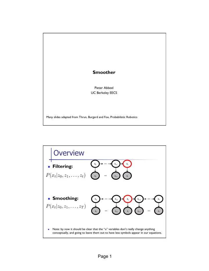
Smoother Pieter Abbeel UC Berkeley EECS Many slides adapted from Thrun, Burgard and Fox, Probabilistic Robotics Overview X 0 X t-1 X t n Filtering: z 0 z t-1 z t n Smoothing: X 0 X t-1 X t X t+1 X T z 0 z t-1 z t z t+1 z T Note: by now it should be clear that the “u” variables don’t really change anything n conceptually, and going to leave them out to have less symbols appear in our equations. Page 1 �

Filtering n Generally, recursively compute: Smoothing Generally, recursively compute: n n Forward: (same as filter) n Backward: n Combine: Page 2 �

Complete Smoother Algorithm n Forward pass (= filter): n Backward pass: n Combine: Note 1: computes for all times t in one forward+backward pass Note 2: can find P( x t | z 0 , …, z T ) by simply renormalizing Important Variation n Find n Recall: n So we can readily compute (Law of total probability) (Markov assumptions) (definitions a, b) Page 3 �

Exercise n Find Kalman Smoother n = smoother we just covered instantiated for the particular case when P( x t+1 | x t ) and P( z t | x t ) are linear Gaussians n We already know how to compute the forward pass (=Kalman filtering) n Backward pass: n Combination: Page 4 �

Kalman Smoother Backward Pass n TODO: work out integral for b t n TODO: insert backward pass update equations n TODO: insert combination à bring renormalization constant up front so it’s easy to read off P( x t | z 0 , …, z T ) Matlab code data generation example A = [ 0.99 0.0074; -0.0136 0.99]; C = [ 1 1 ; -1 +1]; � n x(:,1) = [-3;2]; � n Sigma_w = diag([.3 .7]); Sigma_v = [2 .05; .05 1.5]; � n w = randn(2,T); w = sqrtm(Sigma_w)*w; v = randn(2,T); v = sqrtm(Sigma_v)*v; � n for t=1:T-1 � n � x(:,t+1) = A * x(:,t) + w(:,t); � � y(:,t) = C*x(:,t) + v(:,t); � � end � % now recover the state from the measurements � n P_0 = diag([100 100]); x0 =[0; 0]; � n % run Kalman filter and smoother here n % + plot n Page 5 �

Kalman filter/smoother example Page 6 �