Outline Notes: Scalar nonlinear conservation laws Traffic flow - PDF document

Outline Notes: • Scalar nonlinear conservation laws • Traffic flow • Shocks and rarefaction waves • Burgers’ equation • Rankine-Hugoniot conditions • Importance of conservation form • Weak solutions Reading: Chapter 11, 12 R.J. LeVeque, University of Washington IPDE 2011, June 30, 2011 R.J. LeVeque, University of Washington IPDE 2011, June 30, 2011 Shock formation Notes: For nonlinear problems wave speed generally depends on q . Waves can steepen up and form shocks = ⇒ even smooth data can lead to discontinuous solutions. Note: • System of two equations gives rise to 2 waves. • Each wave behaves like solution of nonlinear scalar equation. R.J. LeVeque, University of Washington IPDE 2011, June 30, 2011 [FVMHP Chap. 13] R.J. LeVeque, University of Washington IPDE 2011, June 30, 2011 [FVMHP Chap. 13] Not quite... no linear superposition. Nonlinear interaction! 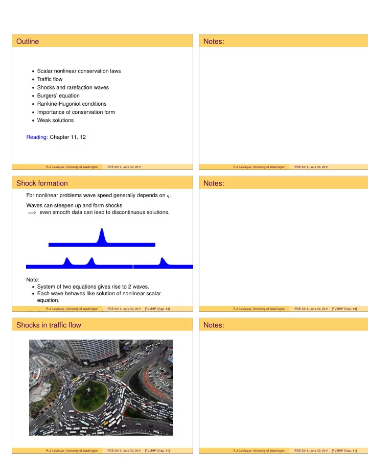Shocks in traffic flow Notes: R.J. LeVeque, University of Washington IPDE 2011, June 30, 2011 [FVMHP Chap. 11] R.J. LeVeque, University of Washington IPDE 2011, June 30, 2011 [FVMHP Chap. 11]

Car following model Notes: X j ( t ) = location of j th car at time t on one-lane road. dX j ( t ) = V j ( t ) . dt Velocity V j ( t ) of j th car varies with j and t . Simple model: Driver adjusts speed (instantly) depending on distance to car ahead. � � V j ( t ) = v X j +1 ( t ) − X j ( t ) for some function v ( s ) that defines speed as a function of separation s . Simulations: http://www.traffic-simulation.de/ R.J. LeVeque, University of Washington IPDE 2011, June 30, 2011 [FVMHP Chap. 11] R.J. LeVeque, University of Washington IPDE 2011, June 30, 2011 [FVMHP Chap. 11] Function v ( s ) (speed as function of separation) Notes: � 1 − L � � u max if s ≥ L, s v ( s ) = 0 if s ≤ L. where: L = car length u max = maximum velocity Local density: 0 < L/s ≤ 1 ( s = L = ⇒ bumper-to-bumper) R.J. LeVeque, University of Washington IPDE 2011, June 30, 2011 [FVMHP Chap. 11] R.J. LeVeque, University of Washington IPDE 2011, June 30, 2011 [FVMHP Chap. 11] Continuum model Notes: Switch to density function: Let q ( x, t ) = density of cars, normalized so: Units for x : carlengths, so x = 10 is 10 carlengths from x = 0 . Units for q : cars per carlength, so 0 ≤ q ≤ 1 . Total number of cars in interval x 1 ≤ x ≤ x 2 at time t is � x 2 q ( x, t ) dx x 1 R.J. LeVeque, University of Washington IPDE 2011, June 30, 2011 [FVMHP Chap. 11] R.J. LeVeque, University of Washington IPDE 2011, June 30, 2011 [FVMHP Chap. 11]

Flux function for traffic Notes: q ( x, t ) = density, u ( x, t ) = velocity = U ( q ( x, t )) . flux: f ( q ) = uq Conservation law: q t + f ( q ) x = 0 . Constant velocity u max independent of density: f ( q ) = u max q = ⇒ q t + u max q x = 0 (advection) Velocity varying with density: V ( s ) = u max (1 − L/s ) = ⇒ U ( q ) = u max (1 − q ) , f ( q ) = u max q (1 − q ) (quadratic nonlinearity) R.J. LeVeque, University of Washington IPDE 2011, June 30, 2011 [FVMHP Chap. 11] R.J. LeVeque, University of Washington IPDE 2011, June 30, 2011 [FVMHP Chap. 11] Characteristics for a scalar problem Notes: q t + f ( q ) x = 0 = ⇒ q t + f ′ ( q ) q x = 0 (if solution is smooth). Characteristic curves satisfy X ′ ( t ) = f ′ ( q ( X ( t ) , t )) , X (0) = x 0 . How does solution vary along this curve? d dtq ( X ( t ) , t ) = q x ( X ( t ) , t ) X ′ ( t ) + q t ( X ( t ) , t ) = q x ( X ( t ) , t ) f ( q ( X ( t ) , t )) + q t ( X ( t ) , t ) = 0 So solution is constant on characteristic as long as solution stays smooth. q ( X ( t ) , t ) = constant = ⇒ X ′ ( t ) is constant on characteristic, so characteristics are straight lines! R.J. LeVeque, University of Washington IPDE 2011, June 30, 2011 [FVMHP Chap. 11] R.J. LeVeque, University of Washington IPDE 2011, June 30, 2011 [FVMHP Chap. 11] Nonlinear Burgers’ equation Notes: � 1 2 u 2 � f ( u ) = 1 2 u 2 . Conservation form: u t + x = 0 , Quasi-linear form: u t + uu x = 0 . This looks like an advection equation with u advected with speed u . True solution: u is constant along characteristic with speed f ′ ( u ) = u until the wave “breaks” (shock forms). R.J. LeVeque, University of Washington IPDE 2011, June 30, 2011 [FVMHP Chap. 11] R.J. LeVeque, University of Washington IPDE 2011, June 30, 2011 [FVMHP Chap. 11]

Burgers’ equation Notes: The solution is constant on characteristics so each value advects at constant speed equal to the value... R.J. LeVeque, University of Washington IPDE 2011, June 30, 2011 [FVMHP Chap. 11] R.J. LeVeque, University of Washington IPDE 2011, June 30, 2011 [FVMHP Chap. 11] Burgers’ equation Notes: Equal-area rule: The area “under” the curve is conserved with time, We must insert a shock so the two areas cut off are equal. R.J. LeVeque, University of Washington IPDE 2011, June 30, 2011 [FVMHP Chap. 11] R.J. LeVeque, University of Washington IPDE 2011, June 30, 2011 [FVMHP Chap. 11] Vanishing Viscosity solution Notes: � 1 2 u 2 � Viscous Burgers’ equation: u t + x = ǫu xx . This parabolic equation has a smooth C ∞ solution for all t > 0 for any initial data. Limiting solution as ǫ → 0 gives the shock-wave solution. Why try to solve hyperbolic equation? • Solving parabolic equation requires implicit method, • Often correct value of physical “viscosity” is very small, shock profile that cannot be resolved on the desired grid = ⇒ smoothness of exact solution doesn’t help! R.J. LeVeque, University of Washington IPDE 2011, June 30, 2011 [FVMHP Chap. 11] R.J. LeVeque, University of Washington IPDE 2011, June 30, 2011 [FVMHP Chap. 11]

Discontinuous solutions Notes: Vanishing Viscosity solution: The Riemann solution q ( x, t ) is the limit as ǫ → 0 of the solution q ǫ ( x, t ) of the parabolic advection-diffusion equation q t + uq x = ǫq xx . For any ǫ > 0 this has a classical smooth solution: R.J. LeVeque, University of Washington IPDE 2011, June 30, 2011 [FVMHP Sec. 11.11 ] R.J. LeVeque, University of Washington IPDE 2011, June 30, 2011 [FVMHP Sec. 11.11 ] Weak solutions to q t + f ( q ) x = 0 Notes: q ( x, t ) is a weak solution if it satisfies the integral form of the conservation law over all rectangles in space-time, � x 2 � x 2 q ( x, t 2 ) dx − q ( x, t 1 ) dx x 1 x 1 � t 2 � t 2 = f ( q ( x 1 , t )) dt − f ( q ( x 2 , t )) dt t 1 t 1 Obtained by integrating � x 2 d q ( x, t ) dx = f ( q ( x 1 , t )) − f ( q ( x 2 , t )) dt x 1 from t n to t n +1 . R.J. LeVeque, University of Washington IPDE 2011, June 30, 2011 [FVMHP Sec. 11.11] R.J. LeVeque, University of Washington IPDE 2011, June 30, 2011 [FVMHP Sec. 11.11] Weak solutions to q t + f ( q ) x = 0 Notes: Alternatively, multiply PDE by smooth test function φ ( x, t ) , with compact support ( φ ( x, t ) ≡ 0 for | x | and t sufficiently large), and then integrate over rectangle, � ∞ � ∞ � � q t + f ( q ) x φ ( x, t ) dx dt 0 −∞ Then we can integrate by parts to get � ∞ � ∞ � ∞ � � qφ t + f ( q ) φ x dx dt = − q ( x, 0) φ ( x, 0) dx. 0 0 −∞ q ( x, t ) is a weak solution if this holds for all such φ . R.J. LeVeque, University of Washington IPDE 2011, June 30, 2011 [FVMHP Sec. 11.11] R.J. LeVeque, University of Washington IPDE 2011, June 30, 2011 [FVMHP Sec. 11.11]

Weak solutions to q t + f ( q ) x = 0 Notes: A function q ( x, t ) that is piecewise smooth with jump discontinuities is a weak solution only if: • The PDE is satisfied where q is smooth, • The jump discontinuities all satisfy the Rankine-Hugoniot conditions. Note: The weak solution may not be unique! R.J. LeVeque, University of Washington IPDE 2011, June 30, 2011 [FVMHP Sec. 11.11] R.J. LeVeque, University of Washington IPDE 2011, June 30, 2011 [FVMHP Sec. 11.11] Shock speed with states q l and q r at instant t 1 Notes: shock with speed s t 1 + ∆ t q = q r q = q l t 1 x 1 x 1 + ∆ x Then Z x 1 +∆ x Z x 1 +∆ x q ( x, t 1 + ∆ t ) dx − q ( x, t 1 ) dx x 1 x 1 Z t 1 +∆ t Z t 1 +∆ t = f ( q ( x 1 , t )) dt − f ( q ( x 1 + ∆ x, t )) dt. t 1 t 1 Since q is essentially constant along each edge, this becomes ∆ x q l − ∆ x q r = ∆ tf ( q l ) − ∆ tf ( q r ) + O (∆ t 2 ) , Taking the limit as ∆ t → 0 gives s ( q r − q l ) = f ( q r ) − f ( q l ) . R.J. LeVeque, University of Washington IPDE 2011, June 30, 2011 [FVMHP Sec. 11.11 ] R.J. LeVeque, University of Washington IPDE 2011, June 30, 2011 [FVMHP Sec. 11.11 ] Rankine-Hugoniot jump condition Notes: s ( q r − q l ) = f ( q r ) − f ( q l ) . This must hold for any discontinuity propagating with speed s , even for systems of conservation laws. For scalar problem, any jump allowed with speed: s = f ( q r ) − f ( q l ) . q r − q l For systems, q r − q l and f ( q r ) − f ( q l ) are vectors, s scalar, R-H condition: f ( q r ) − f ( q l ) must be scalar multiple of q r − q l . For linear system, f ( q ) = Aq , this says A ( q r − q l ) = s ( q r − q l ) , Jump must be an eigenvector, speed s the eigenvalue. R.J. LeVeque, University of Washington IPDE 2011, June 30, 2011 [FVMHP Sec. 11.11 ] R.J. LeVeque, University of Washington IPDE 2011, June 30, 2011 [FVMHP Sec. 11.11 ]