Outline CS 188: Artificial Intelligence Markov Decision Processes - PDF document

Outline CS 188: Artificial Intelligence § Markov Decision Processes (MDPs) § Formalism § Value iteration Markov Decision Processes (MDPs) § In essence a graph search version of expectimax, but § there are rewards in every step (rather than a utility just in the terminal node) § ran bottom-up (rather than recursively) § can handle infinite duration games § Policy Evaluation and Policy Iteration Pieter Abbeel – UC Berkeley Some slides adapted from Dan Klein 1 2 Non-Deterministic Search Grid World § The agent lives in a grid How do you plan when your actions might fail? 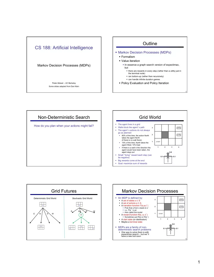§ Walls block the agent ’ s path § The agent ’ s actions do not always go as planned: § 80% of the time, the action North takes the agent North (if there is no wall there) § 10% of the time, North takes the agent West; 10% East § If there is a wall in the direction the agent would have been taken, the agent stays put § Small “ living ” reward each step (can be negative) § Big rewards come at the end § Goal: maximize sum of rewards 3 Grid Futures Markov Decision Processes § An MDP is defined by: Deterministic Grid World Stochastic Grid World § A set of states s ∈ S § A set of actions a ∈ A § A transition function T(s,a,s ’ ) X X § Prob that a from s leads to s ’ § i.e., P(s ’ | s,a) E N S W § Also called the model E N S W § A reward function R(s, a, s ’ ) ? § Sometimes just R(s) or R(s ’ ) § A start state (or distribution) § Maybe a terminal state X X § MDPs are a family of non- X X deterministic search problems § One way to solve them is with expectimax search – but we ’ ll have a new tool soon 5 6 1

What is Markov about MDPs? Solving MDPs § In deterministic single-agent search problems, want an § Andrey Markov (1856-1922) optimal plan, or sequence of actions, from start to a goal § In an MDP, we want an optimal policy π *: S → A § “ Markov ” generally means that given the present state, the future and the § A policy π gives an action for each state § An optimal policy maximizes expected utility if followed past are independent § Defines a reflex agent § For Markov decision processes, “ Markov ” means: Optimal policy when R (s, a, s ’ ) = -0.03 for all non-terminals s Example Optimal Policies Example: High-Low § Three card types: 2, 3, 4 § Infinite deck, twice as many 2 ’ s § Start with 3 showing § After each card, you say “ high ” 3 or “ low ” 4 § New card is flipped 2 § If you ’ re right, you win the R(s) = -0.01 R(s) = -0.03 points shown on the new card 2 § Ties are no-ops § If you ’ re wrong, game ends § Differences from expectimax: § #1: get rewards as you go --- could modify to pass the sum up You can patch expectimax to deal with #1 exactly, but § #2: you might play forever! --- would need to prune those, we’ll not #2 … R(s) = -0.4 R(s) = -2.0 see a better way 9 10 High-Low as an MDP Example: High-Low § States: 2, 3, 4, done 3 § Actions: High, Low § Model: T(s, a, s ’ ): High Low § P(s ’ =4 | 4, Low) = 1/4 3 § P(s ’ =3 | 4, Low) = 1/4 4 3 3 § P(s ’ =2 | 4, Low) = 1/2 2 , Low , High § P(s ’ =done | 4, Low) = 0 § P(s ’ =4 | 4, High) = 1/4 2 § P(s ’ =3 | 4, High) = 0 T = 0.5, T = 0.25, T = 0, T = 0.25, § P(s ’ =2 | 4, High) = 0 R = 3 R = 4 R = 0 R = 2 § P(s ’ =done | 4, High) = 3/4 § … 2 3 4 § Rewards: R(s, a, s ’ ): § Number shown on s ’ if s ≠ s ’ § 0 otherwise Low High Low Low High High § Start: 3 12 2

MDP Search Trees Utilities of Sequences § Each MDP state gives an expectimax-like search tree § What utility does a sequence of rewards have? s is a state § Formally, we generally assume stationary preferences: s a (s, a) is a s, a q-state (s,a,s ’ ) called a transition § Theorem: only two ways to define stationary utilities T(s,a,s ’ ) = P(s ’ |s,a) s,a,s ’ § Additive utility: R(s,a,s ’ ) s ’ § Discounted utility: 13 14 Infinite Utilities?! Discounting § Problem: infinite state sequences have infinite rewards § Typically discount rewards by γ < 1 each time step § Solutions: § Sooner rewards have higher utility than later rewards § Finite horizon: § Also helps the algorithms § Terminate episodes after a fixed T steps (e.g. life) converge § Gives nonstationary policies ( π depends on time left) § Absorbing state: guarantee that for every policy, a terminal state will eventually be reached (like “ done ” for High-Low) § Example: discount of 0.5 § Discounting: for 0 < γ < 1 § U([1,2,3]) = 1*1 + 0.5*2 + 0.25*3 § U([1,2,3]) < U([3,2,1]) § Smaller γ means smaller “ horizon ” – shorter term focus 15 16 Recap: Defining MDPs Our Status § Markov decision processes: § Markov Decision Processes (MDPs) s § States S § Formalism a § Start state s 0 s, a § Actions A § Value iteration § Transitions P(s ’ |s,a) (or T(s,a,s ’ )) s,a,s ’ § In essence a graph search version of expectimax, § Rewards R(s,a,s ’ ) (and discount γ ) s but ’ § there are rewards in every step (rather than a utility just in § MDP quantities so far: the terminal node) § ran bottom-up (rather than recursively) § Policy = Choice of action for each state § can handle infinite duration games § Utility (or return) = sum of discounted rewards § Policy Evaluation and Policy Iteration 17 18 3

Expectimax for an MDP Expectimax for an MDP Example MDP used for illustration has two states, S = {A, B}, and two actions, A = {1, 2} Example MDP used for illustration has two states, S = {A, B}, and two actions, A = {1, 2} i=number of time-steps left state A S i=3 state B A Q state (A,1) Q i=3 Q state (A,2) R,T S i=2 Q state (B,1) A Q state (B,2) i=2 Q Q R,T R,T S i=1 S A A i=1 Q Q R,T R,T S S i=0 19 21 Expectimax for an MDP Expectimax for an MDP Example MDP used for illustration has two states, S = {A, B}, and two actions, A = {1, 2} Example MDP used for illustration has two states, S = {A, B}, and two actions, A = {1, 2} i=number of time-steps left state A i=number of time-steps left state A i=3 i=3 state B state B Q state (A,1) Q state (A,1) i=3 i=3 Q state (A,2) Q state (A,2) i=2 Q state (B,1) i=2 Q state (B,1) Q state (B,2) Q state (B,2) i=2 i=2 Q Q R,T R,T i=1 S i=1 S A A i=1 i=1 Q Q R,T R,T S S i=0 i=0 22 23 Expectimax for an MDP Expectimax for an MDP Example MDP used for illustration has two states, S = {A, B}, and two actions, A = {1, 2} Example MDP used for illustration has two states, S = {A, B}, and two actions, A = {1, 2} i=number of time-steps left state A i=number of time-steps left state A i=3 i=3 state B state B Q state (A,1) Q state (A,1) i=3 i=3 Q state (A,2) Q state (A,2) Q state (B,1) Q state (B,1) i=2 i=2 Q state (B,2) Q state (B,2) i=2 i=2 Q Q R,T R,T i=1 S i=1 S A A i=1 i=1 Q Q R,T R,T S S i=0 i=0 24 25 4

Expectimax for an MDP Expectimax for an MDP Example MDP used for illustration has two states, S = {A, B}, and two actions, A = {1, 2} Example MDP used for illustration has two states, S = {A, B}, and two actions, A = {1, 2} i=number of time-steps left state A i=number of time-steps left state A i=3 i=3 state B state B Q state (A,1) Q state (A,1) i=3 i=3 Q state (A,2) Q state (A,2) i=2 Q state (B,1) i=2 Q state (B,1) Q state (B,2) Q state (B,2) i=2 i=2 Q Q R,T R,T i=1 S i=1 S A A i=1 i=1 Q Q R,T R,T S S i=0 i=0 26 27 Expectimax for an MDP Value Iteration Performs this Q state (A,2) state A state B Computation Bottom to Top Q state (B,1) Example MDP used for illustration has two states, S = {A, B}, and two actions, A = {1, 2} Q state (A,1) Q state (B,2) Example MDP used for illustration has two states, S = {A, B}, and two actions, A = {1, 2} i=number of time-steps left state A i=number of time-steps left i=3 i=3 state B Q state (A,1) i=3 i=3 Q state (A,2) i=2 Q state (B,1) i=2 Q state (B,2) i=2 i=2 Q R,T i=1 S i=1 A i=1 i=1 Q R,T S i=0 i=0 Initialization: 28 29 Value Iteration for Finite Horizon Value Iteration for Finite Horizon H and no Discounting H and with Discounting § Initialization: § Initialization: § For i =1, 2, … , H § For i =1, 2, … , H § For all s 2 S § For all s 2 S § For all a 2 A: § For all a 2 A: § § § V *i (s) : the expected sum of rewards accumulated when starting from § V *i (s) : the expected sum of discounted rewards accumulated when state s and acting optimally for a horizon of i time steps. starting from state s and acting optimally for a horizon of i time steps. § Q *i (s): the expected sum of rewards accumulated when starting from § Q *i (s): the expected sum of discounted rewards accumulated when state s with i time steps left, and when first taking action and acting starting from state s with i time steps left, and when first taking action optimally from then onwards and acting optimally from then onwards § How to act optimally? Follow optimal policy ¼ * i (s) when i steps remain: § How to act optimally? Follow optimal policy ¼ * i (s) when i steps remain: 30 31 5