Occupancy Grid Map Lecture 13: Occupancy Grids CS 344R/393R: - PDF document

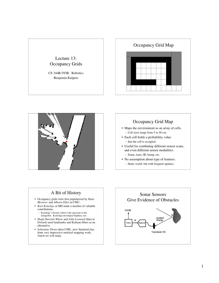
Occupancy Grid Map Lecture 13: Occupancy Grids CS 344R/393R: Robotics Benjamin Kuipers Occupancy Grid Map • Maps the environment as an array of cells. – Cell sizes range from 5 to 50 cm. • Each cell holds a probability value – that the cell is occupied. • Useful for combining different sensor scans, and even different sensor modalities. – Sonar, laser, IR, bump, etc. • No assumption about type of features. – Static world, but with frequent updates. A Bit of History Sonar Sensors • Occupancy grids were first popularized by Hans Give Evidence of Obstacles Moravec and Alberto Elfes at CMU. • Kurt Konolige at SRI made a number of valuable contributions. – Konolige’s Erratic robot is the ancestor to the Amigobot. Konolige developed Saphira, too. • Hugh Durrant-Whyte and John Leonard (then at Oxford) used landmarks and Kalman filters as an alternative. • Sebastian Thrun (then CMU, now Stanford) has done very impressive metrical mapping work, which we will study. 1

Sonar Sweeps Occupancy from Sonar Return a Wide Cone • One 2D Gaussian • Obstacle could be for information anywhere on the arc about occupancy. at distance D. • The space closer than • Another for free D is likely to be free. space. Diffuse and Specular Reflections Wide Sonar Cone Creates a Noisy Map • Diffuse • Specular • From Moravec [1988] Specular Reflections in Sonar Laser Range Finder • Specular (multi-path) reflections hallucinate free space. • 180 ranges over 180 ° planar field of view • 10-12 scans/second • 4 cm range resolution • Max range 50-80 m. • Problems with mirrors, glass, and matte black. • Much better than sonar! 2

Laser Rangefinder Image • 180 narrow beams at 1º intervals. Probabilistic Occupancy Grids Occupancy Grid Cells C ij • The proposition occ ( i,j ) means: • We will apply Bayes Law – The cell C ij is occupied. p ( A | B ) = p ( B | A ) � p ( A ) • Probability : p ( occ ( i,j )) has range [0,1]. p ( B ) • Odds : o ( occ ( i,j )) has range [0,+ ∞ ). – where A is occ ( i,j ) o ( A ) = p ( A ) – and B is an observation r = D p ( ¬ A ) • Log odds : log o ( occ ( i,j )) has range ( −∞ ,+ ∞ ) • We can simplify this by using the log odds • Each cell C ij holds the value log o ( occ ( i,j )) representation. – C ij = 0 corresponds to p ( occ ( i,j )) = 0.5 Bayes Law Using Odds Easy Update Using Bayes Law p ( A | B ) = p ( B | A ) � p ( A ) • Bayes Law: • Bayes’ Law can be written: p ( B ) o ( A | B ) = � ( B | A ) � o ( A ) p ( ¬ A | B ) = p ( B | ¬ A ) � p ( ¬ A ) • Likewise: p ( B ) • Take log odds to make multiplication into o ( A | B ) = p ( A | B ) p ( B | A ) � p ( A ) addition. • so: p ( ¬ A | B ) = p ( B | ¬ A )* p ( ¬ A ) log o ( A | B ) = log � ( B | A ) + log o ( A ) = � ( B | A )* o ( A ) • where: • Easy update for cell contents. o ( A | B ) = p ( A | B ) � ( B | A ) = p ( B | A ) p ( ¬ A | B ) p ( B | ¬ A ) 3

Sensor Model p ( r=D | occ ( i,j )) Occupancy Grid Cell Update • Cell C ij holds log o ( occ ( i,j )). • Probability of range-reading given known occupancy at a known distance. • Evidence r=D means sensor r returns D . • For each cell C ij accumulate evidence from each sensor reading. log o ( A | B ) = log � ( B | A ) + log o ( A ) log o ( occ ( i , j )) + log � ( r = D | occ ( i , j )) = log o ( occ ( i , j ) | r = D ) Mapping One Laser Scan Update Values for λ • If the laser terminates at C ij at distance D � ( r = D | occ ( i , j )) = p ( r = D | occ ( i , j )) p ( r = D | ¬ occ ( i , j )) � .06 .005 = 12 – so log 2 λ ≈ +3.5 • If the laser passes through C ij . � ( r > D | occ ( i , j )) = p ( r > D | occ ( i , j )) p ( r > D | ¬ occ ( i , j )) � .45 .90 = .5 – so log 2 λ ≈ − 1.0 Future Attraction: SLAM Mapping Assignments (4 and 5) • To build an accurate map, we assume that • We will give you laser range-sensor traces. robot pose ( x,y, θ ) is known accurately. – Few specular reflections; no spreading cone. – This is usually not true. – Off-line computation; no physical control. • Localization means using sensor input to • For Assignment 4 , you will have accurate estimate the robot pose ( x,y, θ ). pose information ( x,y, θ ). • Simultaneous Localization and Mapping – You build an accurate occupancy grid map. (SLAM) uses the existing map and current • For Assignment 5 , you will do simultaneous sensor input for localization. localization and mapping (SLAM). – Once localized, use sensors to update the map – You are given laser and odometry sensor values. 4

Implementation Hints Implementation Hints • Use 10 × 10 cm 2 grid cells. • Robot pose ( x,y, θ ) and laser endpoints ( p,q ) are high-resolution values. – But make cell size a parameter and try others. – Grid cells correspond to extended regions. • To display the grid: • Put cell centers at integer coordinates so – Black means occupied rounding quickly gives cell coordinates. – White means free – Grey means unknown • Increment C ij for endpoint of laser beam. • Experiment with different shade mappings. • Step regularly along free part of the beam, decrementing C ij for free cells. – Make it both useful and attractive. 5