Objective Cluster Identification A Finite State Machine Approach - - PowerPoint PPT Presentation

A Finite State Machine Approach to Cluster Identification Using the Hoshen-Kopelman Algorithm

Matthew Aldridge

Objective

• Want to find and identify homogeneous

patches in a 2D matrix, where:

• Cluster membership defined by adjacency
• No need for distance function
• Sequential cluster IDs not necessary

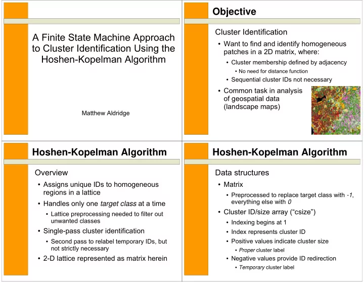
Cluster Identification

• Common task in analysis
• f geospatial data

(landscape maps)

Hoshen-Kopelman Algorithm

• Assigns unique IDs to homogeneous

regions in a lattice

• Handles only one target class at a time
• Lattice preprocessing needed to filter out

unwanted classes

• Single-pass cluster identification
• Second pass to relabel temporary IDs, but

not strictly necessary

• 2-D lattice represented as matrix herein

Overview

Hoshen-Kopelman Algorithm

• Matrix
• Preprocessed to replace target class with -1,

everything else with 0

• Cluster ID/size array (“csize”)
• Indexing begins at 1
• Index represents cluster ID
• Positive values indicate cluster size
• Proper cluster label
• Negative values provide ID redirection
• Temporary cluster label

Data structures

Hoshen-Kopelman Algorithm

csize array

1 6 5 4 3 2 7

• 3

5 8

• 1

4 1

• + values: cluster size
• Cluster 2 has 8 members
• - values: ID redirection
• Cluster 4 is the same as

cluster 1, same as cluster 3

• Cluster 4/1/3 has 5 members
• Redirection allowed for

noncircular, recursive path for finite number of steps

Hoshen-Kopelman Algorithm

• Matrix traversed row-wise
• If current cell nonzero
• Search for nonzero (target class) neighbors
• If no nonzero neighbors found ...
• Give cell new label
• Else ...
• Find proper labels K of nonzero neighbor cells
• min(K) is the new proper label for current cell

and nonzero neighbors

Clustering procedure

Hoshen-Kopelman Algorithm

• North/East/West/South neighbors
• Used in classic HK implementations
• Of the four neighbors, only N/W have

been previously labeled at any given time

Nearest-Four Neighborhood

i, j i, j-1 C N E S W i, j+1 i+1, j i-1, j

Hoshen-Kopelman Algorithm

Nearest-4 HK in action...

• Matrix has been preprocessed
• Target class value(s) replaced with -1, all
• thers with 0

1

• 1
• 1
• 1
• 1
• 1
• 1
• 1
• 1
• 1
• 1
• 1
• 1
• 1
• 1
• 1
• 1
• 1
• 1
• 1
• 1
• 1
• 1
• 1
• 1
• 1
• 1
• 1
• 1
• 1
• 1
• 1
• 1
• 1
• 1
• 1

2 3 4 5 6 7 8 9 10 11 12

Hoshen-Kopelman Algorithm

Nearest-4 HK in action...

• First row, two options:
• Add top buffer row of zeros, OR
• Ignore N neighbor check

1 1

1 2 3 3

• 1
• 1
• 1
• 1
• 1
• 1
• 1
• 1
• 1
• 1
• 1
• 1
• 1
• 1
• 1
• 1
• 1
• 1
• 1
• 1
• 1
• 1
• 1
• 1
• 1
• 1
• 1
• 1
• 1
• 1
• 1

1 2 2 3 4 5 6 7 8 9 10 11 12

Hoshen-Kopelman Algorithm

Nearest-4 HK in action...

1 1

1 2 3 3

• 1
• 1
• 1
• 1
• 1
• 1
• 1
• 1
• 1
• 1
• 1
• 1
• 1
• 1
• 1
• 1
• 1
• 1
• 1
• 1
• 1
• 1
• 1
• 1
• 1
• 1
• 1
• 1
• 1
• 1
• 1

1 2 2 3 4 5 6 7 8 9 10 11 12

Hoshen-Kopelman Algorithm

Nearest-4 HK in action...

1 2

1 2 3 3 1

• 1
• 1
• 1
• 1
• 1
• 1
• 1
• 1
• 1
• 1
• 1
• 1
• 1
• 1
• 1
• 1
• 1
• 1
• 1
• 1
• 1
• 1
• 1
• 1
• 1
• 1
• 1
• 1
• 1
• 1

1 2 2 3 4 5 6 7 8 9 10 11 12

Hoshen-Kopelman Algorithm

Nearest-4 HK in action...

1 2

1 2 3 3 1

• 1
• 1
• 1
• 1
• 1
• 1
• 1
• 1
• 1
• 1
• 1
• 1
• 1
• 1
• 1
• 1
• 1
• 1
• 1
• 1
• 1
• 1
• 1
• 1
• 1
• 1
• 1
• 1
• 1
• 1

1 2 2 3 4 5 6 7 8 9 10 11 12

Hoshen-Kopelman Algorithm

Nearest-4 HK in action...

1 2

1 2 3 3 1 2

• 1
• 1
• 1
• 1
• 1
• 1
• 1
• 1
• 1
• 1
• 1
• 1
• 1
• 1
• 1
• 1
• 1
• 1
• 1
• 1
• 1
• 1
• 1
• 1
• 1
• 1
• 1
• 1
• 1

2 2 2 3 4 5 6 7 8 9 10 11 12

Hoshen-Kopelman Algorithm

Nearest-4 HK in action...

1 2

1 2 3 3 1 2

• 1
• 1
• 1
• 1
• 1
• 1
• 1
• 1
• 1
• 1
• 1
• 1
• 1
• 1
• 1
• 1
• 1
• 1
• 1
• 1
• 1
• 1
• 1
• 1
• 1
• 1
• 1
• 1
• 1

2 2 2 3 4 5 6 7 8 9 10 11 12

Hoshen-Kopelman Algorithm

Nearest-4 HK in action...

1 2

1 2 3 3 1 2 4

• 1
• 1
• 1
• 1
• 1
• 1
• 1
• 1
• 1
• 1
• 1
• 1
• 1
• 1
• 1
• 1
• 1
• 1
• 1
• 1
• 1
• 1
• 1
• 1
• 1
• 1
• 1
• 1

2 2 1 2 3 4 5 6 7 8 9 10 11 12

Hoshen-Kopelman Algorithm

Nearest-4 HK in action...

1 2

1 2 3 3 1 2 4 3

• 1
• 1
• 1
• 1
• 1
• 1
• 1
• 1
• 1
• 1
• 1
• 1
• 1
• 1
• 1
• 1
• 1
• 1
• 1
• 1
• 1
• 1
• 1
• 1
• 1
• 1
• 1

2 4

• 3

2 3 4 5 6 7 8 9 10 11 12

Hoshen-Kopelman Algorithm

Nearest-4 HK in action...

1 2

1 2 3 3 1 2 4 3

• 1
• 1
• 1
• 1
• 1
• 1
• 1
• 1
• 1
• 1
• 1
• 1
• 1
• 1
• 1
• 1
• 1
• 1
• 1
• 1
• 1
• 1
• 1
• 1
• 1
• 1
• 1

2 4

• 3

2 3 4 5 6 7 8 9 10 11 12

Hoshen-Kopelman Algorithm

Nearest-4 HK in action...

1 2

1 2 3 3 1 2 4 3 5

• 1
• 1
• 1
• 1
• 1
• 1
• 1
• 1
• 1
• 1
• 1
• 1
• 1
• 1
• 1
• 1
• 1
• 1
• 1
• 1
• 1
• 1
• 1
• 1
• 1
• 1

2 4

• 3

1 2 3 4 5 6 7 8 9 10 11 12

Hoshen-Kopelman Algorithm

1 2

1 2 3 3 1 2 4 3 5 5

• 1

2 2 2 2

• 1
• 1
• 1
• 1
• 1
• 1
• 1
• 1
• 1
• 1
• 1
• 1
• 1
• 1
• 1
• 1
• 1
• 1
• 1
• 1

10

• 2
• 3

2 2 3 4 5 6 7 8 9 10 11 12

Nearest-4 HK in action...

Hoshen-Kopelman Algorithm

Nearest-4 HK in action...

1 2

1 2 3 3 1 2 4 3 5 5 5 2 2 2 2 6 6 2 2

• 1
• 1
• 1
• 1
• 1
• 1
• 1
• 1
• 1
• 1
• 1
• 1
• 1
• 1
• 1
• 1

12

• 2
• 3

3 2 2 3 4 5 6 7 8 9 10 11 12

Hoshen-Kopelman Algorithm

Nearest-4 HK in action...

1 2

1 2 3 3 1 2 4 3 5 5 5 2 2 2 2 6 6 2 2 6 6 7 8 9 7 10 7 7 7 11 7 7 7 7 11

12

• 2
• 3

3 3 11 1

• 7
• 7

2 2 3 4 5 6 7 8 9 10 11 12

• Skipping ahead

Hoshen-Kopelman Algorithm

Nearest-4 HK in action...

1 2

1 2 2 2 1 2 2 2 5 5 5 2 2 2 2 6 6 2 2 6 6 7 8 7 7 7 7 7 7 11 7 7 7 7 11

12

• 2
• 3

3 3 11 1

• 7
• 7

2 2 3 4 5 6 7 8 9 10 11 12

• Optional second pass to relabel cells to

their proper labels

Hoshen-Kopelman Algorithm

• NW, N, NE, E, SE, S, SW, W
• When examining a cell, compare to W,

NW, N, NE neighbors

Nearest-Eight Neighborhood

i, j i, j-1

C N E S W

i, j+1 i+1, j i-1, j i-1, j-1 i-1, j+1

i+1, j+1 i+1, j-1

NW NE SW SE

Hoshen-Kopelman Algorithm

• Sometimes more appropriate in

landscape analysis

• Rasterization can segment continuous

features if only using nearest-four neighborhood

Nearest-Eight Neighborhood

Hoshen-Kopelman Algorithm

Nearest-4 vs. Nearest-8 Results

1 2 2 2 1 2 2 2 5 5 5 2 2 2 2 6 6 2 2 6 6 7 8 7 7 7 7 7 7 11 7 7 7 7 11 1 2 2 2 1 2 2 2 2 2 2 2 2 2 2 2 2 2 2 2 2 2 2 2 2 2 2 2 2 5 2 2 2 2 5

UNION-FIND Algorithm

Disjoint-Set Data Structure

• Maintains collection of non-overlapping

sets of objects

• Each set identifiable by a single

representative object

• Rep. may change as set changes, but

remains the same as long as set unchanged

• Disjoint-set forest is a type of D-S data

structure with sets represented by rooted trees

• Root of tree is representative

UNION-FIND Algorithm

Disjoint-Set Data Structure Operations

• MAKE-SET(x)
• Creates a new set whose only member is x
• UNION(x, y)
• Combines the two sets containing objects x

and y

• FIND-SET(x)
• Returns the representative of the set

containing object x

• An algorithm that performs these ops is

known as a UNION-FIND algorithm

UNION-FIND Algorithm

HK relation to UNION-FIND

• csize array may be viewed as a disjoint-

set forest

1 2 12

• 2
• 3

3 3 11 1

• 7
• 7

2 2 3 4 5 6 7 8 9 10 11 12

2 1 3 4 5 6 7 8 9 10 11

UNION-FIND Algorithm

HK relation to UNION-FIND

• Implementation of UNION-FIND
• perations
• MAKE-SET: When a cell is given a new

label and new cluster is formed

• UNION: When two clusters are merged
• FIND-SET: Also when two clusters are

merged (must determine that the proper labels of the two clusters differ)

UNION-FIND Algorithm

Heuristics to improve UNION-FIND

• Path compression
• Used in FIND-SET to set each node's parent

link to the root/representative node

• FIND-SET becomes two-pass method

1) Follow parent path of x to find root node 2) Traverse back down path and set each node's parent pointer to root node

UNION-FIND Algorithm

Heuristics to improve UNION-FIND

• Union by rank
• Goal: When performing UNION, set root of

smaller tree to point to root of larger tree

• Size of trees not explicitly tracked; rather, a

rank metric is maintained

• Rank is upper bound on height of a node
• MAKE-SET: Set rank of node to 0
• UNION: Root with higher node becomes

parent; in case of tie, choose arbitrarily and increase winner's rank by 1

UNION-FIND Algorithm

Applying these heuristics to HK

• Original HK did not use either heuristic
• Previous FSM implementation

(Constantin, et al.) used only path compression

• Implementation in this study uses path

compression and union by cluster size

• U by cluster size: Similar to U by rank, but

considers size of cluster represented by tree, not size of tree itself

• Reduces the number of relabeling ops in 2nd pass

Finite State Machines

• Set of states
• Each state stores some form of input history
• Input alphabet (set of symbols)
• Input is read by FSM sequentially
• State transition rules
• Next state determined by current state and

current input symbol

• Need rule for every state/input combination

Computational model composed of:

Finite State Machines

• S: Set of states
• Σ: Input alphabet
• Input is read by FSM sequentially
• δ: State transition rules
• (δ: S x Σ → S)
• q0: Starting state
• F: Set of final states

Formal definition: (S, Σ, δ, q0, F)

Nearest-8 HK with FSM

Why apply FSM to Nearest-8 HK?

• Want to retain short-term knowledge on

still relevant, previously examined cells

• Helps avoid costly memory accesses
• Recall from Nearest-8 HK that the W,

NW, N, NE neighbors' values are checked when examining each cell

• (only when the current cell is nonzero!)

Nearest-8 HK with FSM

• Note that a cell and its N, NE neighbors

are next cell's W, NW, N neighbors

• Encapsulate what is known about current

cell and N, NE neighbors into next state

• Number of neighbor comparisons can be

reduced by up to 75%

NW N NE E W SW S SE NW N NE E W SW S SE

Nearest-8 HK with FSM

Let's define our state space...

• Current cell value is always checked, thus

always encapsulated in the next state

• Assume current cell value is nonzero
• N, NE neighbor values are checked (along

with NW, but that's irrelevant for next cell)

• This produces four possible states when

examining the next cell:

1 1

= cluster (nonzero) = no cluster (zero)

Nearest-8 HK with FSM

And if current cell is zero?

• Neighbor values are not checked
• But some neighbor knowledge may still be
• retained. Consider:

= cluster (nonzero) = no cluster (zero) Current cell nonzero, neighbors checked Current cell zero, NO neighbors checked = known value (zero or nonzero) = unknown value Even though previous cell was zero, we can retain knowledge of NW neighbor

Nearest-8 HK with FSM

So, after a single zero value...

• We can still retain knowledge of NW

neighbor

• This produces two more states:

= cluster = no cluster = unknown

? ?

Nearest-8 HK with FSM

What about multiple sequential zeros?

Current cell nonzero, neighbors checked Current cell zero, NO neighbors checked Current cell zero, NO neighbors checked Here we do NOT know the NW neighbor value

• This produces one last

state:

? ?

Nearest-8 HK with FSM

Putting it all together...

? ? 1 1 ?

s0 s1 s2 s3 s4 s5 s6

?

= cluster = current = no cluster = unknown

Details...

• Previous slide is missing a final state
• In formal definition, a terminal symbol is

specified, to be located after last cell

• From any state, encountering this symbol leads to

final state

• Implementation does not include final state

explicitly

• Bounds checking used instead

Nearest-8 HK with FSM

More details...

• Row transitions
• If matrix is padded on both sides with buffer

columns of all zeros, FSM will reset to s0 before proceeding to next row

• In actual implementation, no buffer columns
• Again, explicit bounds checking performed
• At beginning of row, FSM reset to s6
• At end of row, last cell handled as special case

Nearest-8 HK with FSM

s6

? ? ?

s0

• Start with first row clustered as before

In action...

Nearest-8 HK with FSM

1 1

1 2 3 3

• 1
• 1
• 1
• 1
• 1

1 2 2 3 4

In action...

Nearest-8 HK with FSM

1 1

1 2 3 3

• 1
• 1
• 1
• 1
• 1

1 2 2 3 4

? ? 1 1 ?

s0 s1 s2 s3 s4 s5 s6

?

= cluster = current = no cluster = unknown

In action...

Nearest-8 HK with FSM

1 2

1 2 3 3 1

• 1
• 1
• 1
• 1

1 2 2 3 4

? ? 1 1 ?

s0 s1 s2 s3 s4 s5 s6

?

= cluster = current = no cluster = unknown

In action...

Nearest-8 HK with FSM

1 2

1 2 3 3 1

• 1
• 1
• 1
• 1

1 2 2 3 4

? ? 1 1 ?

s0 s1 s2 s3 s4 s5 s6

?

= cluster = current = no cluster = unknown

In action...

Nearest-8 HK with FSM

1 2

1 2 3 3 1

• 1
• 1
• 1
• 1

1 2 2 3 4

? ? 1 1 ?

s0 s1 s2 s3 s4 s5 s6

?

= cluster = current = no cluster = unknown

In action...

Nearest-8 HK with FSM

1 2

1 2 3 3 1 2

• 1
• 1
• 1

2 2 2 3 4

? ? 1 1 ?

s0 s1 s2 s3 s4 s5 s6

?

= cluster = current = no cluster = unknown

In action...

Nearest-8 HK with FSM

1 2

1 2 3 3 1 2

• 1
• 1
• 1

1 2 2 3 4

? ? 1 1 ?

s0 s1 s2 s3 s4 s5 s6

?

= cluster = current = no cluster = unknown

In action...

Nearest-8 HK with FSM

1 2

1 2 3 3 1 2

• 1
• 1
• 1

1 2 2 3 4

? ? 1 1 ?

s0 s1 s2 s3 s4 s5 s6

?

= cluster = current = no cluster = unknown

In action...

Nearest-8 HK with FSM

1 2

1 2 3 3 1 2 3

• 1
• 1

1 3 2 3 4

? ? 1 1 ?

s0 s1 s2 s3 s4 s5 s6

?

= cluster = current = no cluster = unknown

In action...

Nearest-8 HK with FSM

1 2

1 2 3 3 1 2 3

• 1
• 1

1 3 2 3 4

? ? 1 1 ?

s0 s1 s2 s3 s4 s5 s6

?

= cluster = current = no cluster = unknown

In action...

Nearest-8 HK with FSM

1 2

1 2 3 3 1 2 3 3

• 1

1 4 2 3 4

? ? 1 1 ?

s0 s1 s2 s3 s4 s5 s6

?

= cluster = current = no cluster = unknown

In action...

Nearest-8 HK with FSM

1 2

1 2 3 3 1 2 3 3

• 1

1 4 2 3 4

? ? 1 1 ?

s0 s1 s2 s3 s4 s5 s6

?

= cluster = current = no cluster = unknown

In action...

Nearest-8 HK with FSM

1 2

1 2 3 3 1 2 3 3

• 1

1 4 2 3 4

? ? 1 1 ?

s0 s1 s2 s3 s4 s5 s6

?

= cluster = current = no cluster = unknown

In action...

Nearest-8 HK with FSM

1 2

1 2 3 3 1 2 3 3 3

1 5 2 3 4

? ? 1 1 ?

s0 s1 s2 s3 s4 s5 s6

?

= cluster = current = no cluster = unknown

Nearest-8 HK with FSM

Alternative Implementations

• Parallel computing
• MPI used for process communication
• Controller/worker design, round-robin job

assignment

• Matrix divided row-wise into s segments
• csize also divided into s segments, with

mutually exclusive cluster ID spaces

• Results merged by controller node
• Minimal speedup, mostly due to staggered I/O
• May be useful for much larger data than used here

Nearest-8 HK with FSM

Alternative Implementations

• Concurrent FSMs
• Identify multiple target classes in single pass
• Each FSM maintains separate state
• No longer in-place
• Must maintain explicit state variables, rather than

separate blocks of execution and implicit state

Workstation Performance

Methodology

• Tests performed on Linux workstation
• 2.4 GHz Intel Xeon
• 8 KB L1 cache
• 512 KB L2 cache
• Timed over complete cluster analysis
• First AND second pass (relabeling)
• File I/O and data structure initialization not

included

• Average time of 40 executions for each

implementation and parameter set

Workstation Performance

Test Data

• One set of 5000x5000 randomly generated

binary matrices

• Target class densities: { 0.05, 0.1, 0.15, ..., 0.95 }
• Three actual land cover maps
• 2771x2814 Fort Benning, 15 classes
• 4300x9891 Tennessee Valley, 21 classes
• 400x500 Yellowstone, 6 classes

Workstation Performance

Random Data Results

Workstation Performance

Random Data Results

Workstation Performance

Random Data Results

Workstation Performance

Random Data Results

Workstation Performance

Fort Benning Data

Workstation Performance

Fort Benning Data Results

Workstation Performance

Fort Benning Data Results

Workstation Performance

Fort Benning Data Results

Workstation Performance

Fort Benning Data Results

Workstation Performance

Tennessee Valley Data

Workstation Performance

Tennessee Valley Data Results

Workstation Performance

Tennessee Valley Data Results

Workstation Performance

Yellowstone Data

Workstation Performance

Yellowstone Data Results

Workstation Performance

Conclusions

• FSM clearly outperforms non-FSM for both

landscape and random data

• Sparse clusters: non-FSM still competitive
• Dense clusters: FSM advantage increases due to

retaining knowledge of neighbor values more often

• Proper merging (using union by cluster size) is

key to performance

Palm PDA Performance

Why a PDA?

• Perhaps FSM can shine in high-latency

memory system

• Conceivable applications include...
• Mobile computing for field researchers
• Cluster analysis in low-powered embedded

systems

Palm PDA Performance

Methodology

• Tests performed on Palm IIIxe
• 16 MHz Motorola Dragonball 68328EZ
• 8MB RAM
• No cache
• Only one run per implementation and

parameter set

• Single-threaded execution gives very little

variation in run times (within 1/100 second

• bserved)
• Very small datasets

Palm PDA Performance

Test Data

• One set of 150x150 randomly generated

binary matrices

• Target class densities: { 0.05, 0.1, 0.15, ..., 0.95 }
• 175x175 segment of Fort Benning map
• 13 target classes

Palm PDA Performance

Random Data Results

Palm PDA Performance

Fort Benning Data Results

Palm PDA Performance

Branching in FSM vs. Non-FSM

non-FSM FSM (dashed lines indicate state-based branching)

Palm PDA Performance

Conclusions

• Non-FSM implementation faster in all cases
• FSM more competitive with higher target class

densities

• Why is the FSM slower?
• Ironically, lack of cache
• Also, reduced program locality and execution

branching

• Adding as little as 1-2 KB of cache can reduce

Palm's effective memory access time by 50% (Carroll, et al.)

In Closing

Possible Future Work

• Extension to three (or higher?) dimensions
• Higher dimensions => more neighbors => many

more states

• Automated FSM construction would ease burden, allow

non-programmers to define custom neighborhood rules

• If effects of complex control logic/branching can

be mitigated, then FSM savings should be great

• FSM adaptation for different data ordering

(e.g. Z- or Morton-order)

• Implement FSM HK in hardware (FPGAs, etc.)