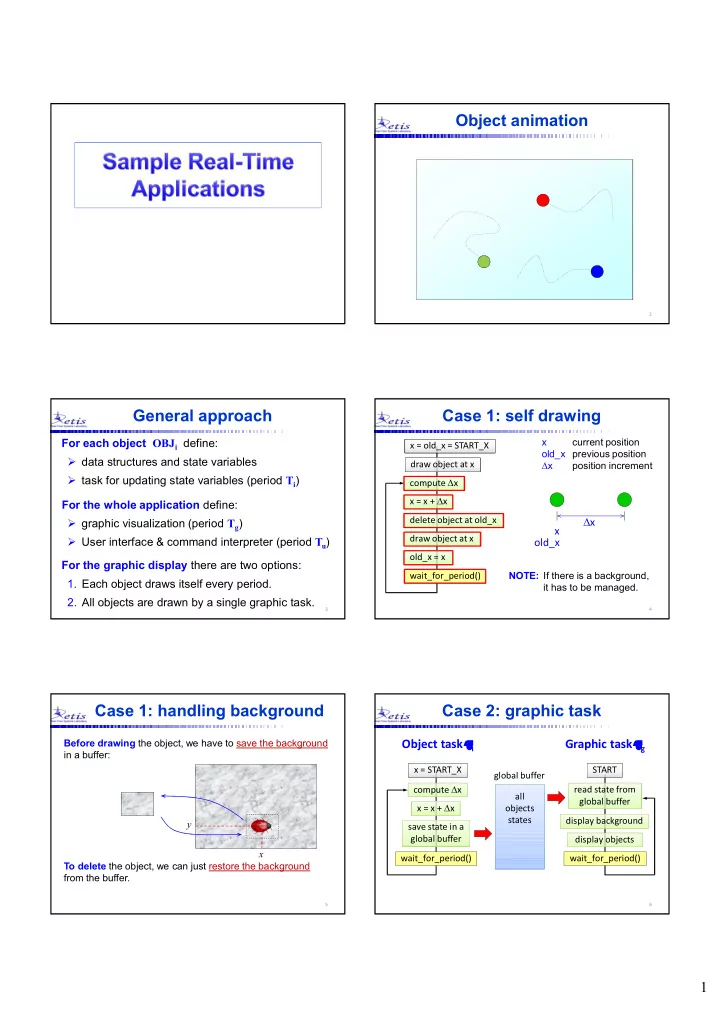
Object animation 2 General approach Case 1: self drawing For each - - PDF document

SLIDE 1

1

2

Object animation

3

General approach

For the graphic display there are two options:

• 1. Each object draws itself every period.
• 2. All objects are drawn by a single graphic task.

For each object OBJi define:

• data structures and state variables
• task for updating state variables (period Ti)

For the whole application define:

• graphic visualization (period Tg)
• User interface & command interpreter (period Tu)

4

Case 1: self drawing

D compute Dx D x = x + Dx delete object at old_x draw object at x

• ld_x = x

wait_for_period() x current position

• ld_x previous position

Dx position increment

x

• ld_x

Dx

x = old_x = START_X draw object at x NOTE: If there is a background, it has to be managed.

5

Case 1: handling background

Before drawing the object, we have to save the background in a buffer: x y To delete the object, we can just restore the background from the buffer.

6

Case 2: graphic task

compute Dx x = x + Dx wait_for_period() x = START_X save state in a global buffer display objects wait_for_period() START read state from global buffer global buffer all

• bjects

states

Object task i Graphic task g

display background

SLIDE 2

2

7

Physical simulations

 Modeling

– Derive the system model expressing the position x as a function of the other state variables.

 Speed must be independent of the period

– compute: dx = vx * T; – For smooth motion, period should be no larger than 20 ms – If T is larger, you can multiply T by a timescale factor.

 Scalability

– Express physical variables in MKS units using floats; – Convert to integer coordinates only for displaying; – use offset and scale factor for graphic coordinates: xg = offset + x * scale;

8

Jumping balls

Let us see how to write a program that simulates a number of jumping balls that move in a box following the laws of physics:

9

Things to define

• General description and requirements
• Application structure
• Graphical layout
• User interface
• Motion rules
• Constants of the simulation
• State variables of the ball
• Global variables and data structures
• Auxiliary functions (divide them into categories)

10

General description

1. Each ball is animated by a dedicated periodic task that updates its state every period. 2. The motion of each ball is independent on the other balls, but depends on its current state. 3. Balls moves within a box and bounce on its borders. 4. Balls lose some energy when bouncing on the floor. 5. The user can interact with the program and can create new balls, make them jumping, vary gravity, etc. 6. The system provides information on: number of active balls, deadline misses, current gravity.

11

Application structure

state var.: (x, y, vx, vy) Ti, Di

i g

Graphics parameters S(t+T)

u

ball task graphic task user task g v0 fixed S(t)

The task animating the ball must periodically update the ball state from S(t) to S(t+T):

12

state array

1

Graphics parameters

i g

state 1 state i

u

user task g v0 Ti, Di

Application structure

graphic task

The state of multiple balls is stored in an array:

SLIDE 3

3

13

Graphical layout

Simulations should be done in real units (MKS) and

• nly later converted in pixels.

Virtual world (meters)

Graphic window Graphic world (pixels)

Menu area

Status window

14

User interface

Inputs

• What variables can the user change?
• Pressing which keys?
• Is the mouse used?

We have to decide the inputs and the outputs: Outputs

• Which variables are displayed?

15

User interface

• SPACE: creates a new ball with random parameters
• ESC: exits the program
• A: makes balls jumping (provide extra energy)
• W: shows/hides the ball trail
• LEFT / RIGHT: decrease/increase trail length
• UP / DOWN: increase/decrease gravity

Corresponding values must be shown on the state window

16

Motion rules

vx (x, y) vy

2

2 1 gt t v y y

curr y curr new

   t v x x

x curr new

 

• These equations must be updated every period Ti
• A time scale can be used for the integration interval:

dt = TSCALE * Ti vx = constant

gt v v

curr y new y

 

18

Makefile

#--------------------------------------------------- # Target file to be compiled by default #--------------------------------------------------- MAIN = balls #--------------------------------------------------- # CC will be the compiler to use #--------------------------------------------------- CC = gcc #--------------------------------------------------- # CFLAGS will be the options passed to the compiler #--------------------------------------------------- CFLAGS = -Wall -lpthread -lrt #--------------------------------------------------- # Dependencies #--------------------------------------------------- $(MAIN): $(MAIN).o ptask.o $(CC) $(CFLAGS) -o $(MAIN) $(MAIN).o ptask.o `allegro-config --libs` $(MAIN).o: $(MAIN).c $(CC) -c $(MAIN).c ptask.o: ptask.c $(CC) -c ptask.c

SLIDE 4

4

19

Header files

//----------------------------------------------------- // BALLS: SIMULATION OF JUMPING BALLS // with a single display task //----------------------------------------------------- #include <stdlib.h> // include standard lib first #include <stdio.h> #include <math.h> #include <pthread.h> #include <sched.h> #include <allegro.h> #include <time.h> #include "ptask.h" // include own lib later #include "mylib.h"

20

Constants

//----------------------------------------------------- // GRAPHICS CONSTANTS //----------------------------------------------------- #define XWIN 640 // window x resolution #define YWIN 480 // window y resolution #define BKG // background color #define MCOL 14 // menu color #define NCOL 7 // numbers color #define TCOL 15 // trail color //----------------------------------------------------- #define LBOX 489 // X length of the ball box #define HBOX 399 // Y height of the ball box #define XBOX 5 // left box X coordinate #define YBOX 75 // upper box Y coordinate #define RBOX 495 // right box X coordinate #define BBOX 475 // bottom box Y coordinate #define FLEV 5 // floor Y level (in world)

21

Constants

//----------------------------------------------------- // TASK CONSTANTS //----------------------------------------------------- #define PER 20 // task period in ms #define DL 20 // relative deadline in ms #define PRI 80 // task priority //----------------------------------------------------- // BALL CONSTANTS //----------------------------------------------------- #define MAX_BALLS 20 // max number of balls #define G0 9.8 // acceleration of gravity #define TLEN 30 // trail length #define HMIN 200 // min initial height #define HMAX 390 // max initial height #define VXMIN 20 // min initial hor. speed #define VXMAX 10 // max initial hor. speed #define DUMP 0.9 // dumping coefficient #define TSCALE 10 // time scale factor

22

State variables

struct status { // ball structure int c; // color [1,15] float r; // radius (m) float x; // x coordinate (m) float y; // y coordinate (m) float vx; // horizontal velocity (m/s) float vy; // vertical velocity (m/s) float v0; // jumping velocity (m/s) }; struct status ball[MAX_BALLS]; // balls status buffer

vx (x,y) color size vy

23

Storing the trail

x1 x2 x3 x4 x5 x6 x1 x2 x3 x4 x5

0 1 2 3 4

top

It can be done using a circular buffer of length L = max trail length:

• top always points to

the most recent data

• next element:

(top + 1) % L

• previous element:

(top – 1 + L) % L

• kth previous element:

(top – k + L) % L

top = (top + 1) % L; cbuf[top] = x;

Store a new value x: cbuf

24

Reading the trail

x1 x2 x3 x4 x5 x6 x6 x2 x3 x4 x5

0 1 2 3 4

top

i = (top – k + L) % L; value = cbuf[i];

Getting the kth previous value :

It can be done using a circular buffer of length L = max trail length:

• top always points to

the most recent data

• next element:

(top + 1) % L

• previous element:

(top – 1 + L) % L

• kth previous element:

(top – k + L) % L

cbuf

SLIDE 5

5

25

Trail functions

struct cbuf { // circular buffer structure int top; // index of the current element int x[TLEN]; // array of x coordinates int y[TLEN]; // array of y coordinates }; struct cbuf trail[MAX_BALLS]; // trail array void store_trail(int i) // insert value of ball i { int k; if (i >= MAX_BALLS) return; k = trail[i].top; k = (k + 1) % TLEN; trail[i].x[k] = ball[i].x; trail[i].y[k] = ball[i].y; trail[i].top = k; }

26

Trail functions

void draw_trail(int i, int w) // draw w past values { int j, k; // trail indexes int x, y; // graphics coordinates for (j=0; j<w; j++) { k = (trail[i].top + TLEN - j) % TLEN; x = XBOX + 1 + trail[i].x[k]; y = YWIN - FLEV - trail[i].y[k]; putpixel(screen, x, y, TCOL); } }

27

Global variables

//----------------------------------------------------- // GLOBAL DATA STRUCTURES //----------------------------------------------------- struct status ball[MAX_BALLS]; // balls buffer struct cbuf trail[MAX_BALLS]; // trail buffer int nab = 0; // number of active balls int tflag = 0; // trail flag int tl = 10; // actual trail length int end = 0; // end flag float g = G0; // acceleration of gravity

28

Auxiliary functions

//---------------------------------------------------- // GET_SCANCODE: returns the scancode of a pressed key //---------------------------------------------------- char get_scancode() { if (keypressed()) return readkey() >> 8; else return 0; }

NOTE: Since the function is non-blocking, returing 0 is crucial to prevent the command interpreter to execute an action multiple times.

Command interpreter

do { scan = get_scancode(); switch (scan) { case KEY_SPACE: if (nab < MAX_BALLS) task_create(nab++, btask, PER, DL,...); break; case KEY_UP: g = g + 1; // increase gravity break; case KEY_DOWN: if (g > 1) g = g - 1; // decrease gravity break; default: break; } } while (scan != KEY_ESC);

30

//------------------------------------------------ // FRAND: returns a random float in [xmi, xma) //------------------------------------------------ float frand(float xmi, float xma) { float r; r = rand()/(float)RAND_MAX; // rand in [0,1) return xmi + (xma - xmi)*r; }

Auxiliary functions

SLIDE 6

6

31

//------------------------------------------------ // DRAW_BALL: draw ball i in graphic coordinates //------------------------------------------------ void draw_ball(int i) { int x, y; x = XBOX + 1 + ball[i].x; y = YWIN - FLEV - ball[i].y; circlefill(screen, x, y, ball[i].r, ball[i].c); }

Auxiliary functions

32

Handling bounces

We need to account for ball dimensions and dumping:

vy =  DUMP * vy

x x

vx =  vx

33

void handle_bounce(int i) { if (ball[i].y <= ball[i].r) { ball[i].y = ball[i].r; ball[i].vy = -DUMP*ball[i].vy; } if (ball[i].y >= HBOX - ball[i].r) { ball[i].y = HBOX - ball[i].r; ball[i].vy = -DUMP*ball[i].vy; } if (ball[i].x >= LBOX - ball[i].r) { ball[i].x = LBOX - ball[i].r; ball[i].vx = -ball[i].vx; } if (ball[i].x <= ball[i].r) { ball[i].x = ball[i].r; ball[i].vx = -ball[i].vx; } }

Handling bounces

34

void init_ball(int i) { int i; // task index ball[i].c = 2 + i%14; // color in [2,15] ball[i].r = frand(RMIN, RMAX); ball[i].x = ball[i].r + 1; ball[i].y = frand(HMIN, HMAX); ball[i].vx = frand(VXMIN, VXMAX); ball[i].vy = 0; ball[i].v0 = sqrt(2*g*ball[i].y); }

Initializing ball status

35

void* balltask(void* arg) { int i; // task index float dt; // integration interval i = task_argument(arg); init_ball(i); dt = TSCALE*(float)task_period(i)/1000; while (!end) { ball[i].vy -= g*dt; ball[i].x += ball[i].vx*dt; ball[i].y += ball[i].vy*dt - g*dt*dt/2; handle_bounce(i); put_trail(i); wait_for_period(i); } }

Ball task

36

void* display(void* arg) { int a; // task index a = task_argument(arg); while (!end) { rectfill(screen, XBOX+1, YBOX+1, RBOX-1, BBOX-1, BKG); for (i=0; i<nab; i++) { draw_ball(i); if (wflag) draw_wake(i, wl); } if (deadline_miss(a)) // check for deadline miss show_dmiss(a); wait_for_period(a); } }

Display task

SLIDE 7

7

37

int main(void) { int i; init(); for (i=0; i<=MAX_BALLS; i++) wait_for_task_end(i); allegro_exit(); return 0; }

Main task

38

void init(void) { int i; char s[20]; allegro_init(); set_gfx_mode(GFX_AUTODETECT_WINDOWED, XWIN, YWIN, 0, 0); clear_to_color(screen, BKG); install_keyboard(); srand(time(NULL)); // initialize random generator // draw menu area // draw box area // draw status area ptask_init(SCHED_FIFO); task_create(MAX_BALLS, display, PER, DREL, PRI1, ACT); task_create(MAX_BALLS+1, interp, PER, DREL, PRI2, ACT); }

Init function

39

Planets simulation

state vector

1

parameters vector

i g

state 1 state i

u

user task g

v0

Ti, Di

Using the same programming structure, we can simulate the behavior of N planets subject to a gravitational field:

k  i

compute dik compute Fik = compute Fi = compute ai = Fi/mi update state (xi, vi) mi mk dik

2

G

 Fik

ik

Task i

41

Random flies

Let us see how to write a program that simulates the motion of a set of flies that move randomly on a given area of the screen:

42

General description

• 1. Each fly should update its state every period.
• 2. Fly motion is independent on the other flies, but

depends on the current speed and direction.

• 3. A fly must bounce on the border of the area.
• 4. The user can create a new fly and vary:

period, zoom, max deviation, max speed, fly shape.

• 5. The system provides information on:

number of created flies, deadline misses, zoom factor.

SLIDE 8

8

43

User interface

The user can create a new fly and vary: period, zoom, max deviation, max speed, fly shape.

• SPACE: create a new fly;
• UP/DOWN arrow: increase/decrease deviation;
• PAD –: zoom in; PAD +: zoom out
• F: change fly shape (toggle)
• D: set default parameters
• ESC exit the program

44

state vector

1 i g

state 1 state i

u

user task  v Ti, Di

Application structure

zoom shape colors size graphic task

45

State variables

struct state // fly structure { int c; // color [1,15] float r; // radius (m) float x; // x coordinate (m) float y; // y coordinate (m) float v; // velocity (m/s) float a; // orientation angle (rad) };

a v (x,y) color size

46

Global variables

struct state fly[MAXFLY]; // fly buffer int naf = 0; // number of active flies float scale = 1; // scale factor float dev = MAXDEV; // deviation factor (deg) float v_max = MAXV; // maximum speed (m/s) int period = PER_F; // period of the fly task int end; // end flag

47

Fly motion rules

vx = | v | cos() vy = | v | sin() Situation at time t

         y x P 

        

y x

v v v 

T v P P       '

dx = vxT



dy = vyT v

          

y x

d y d x P'  P 

Situation at time t+T

48

Fly motion rules

To implement some randomness, v and  can change at every step by a limited amount: Dv and D

P 

+Dv v

• Dv



SLIDE 9

9

49

Fly motion rules

Hence, the position increment can be implemented as follows: +Dv v

• Dv

(x,y)

da = frand(-DELTA_A, DELTA_A); dv = frand(-DELTA_V, DELTA_V); alpha = alpha + da; v = v + dv; vx = v*cos(alpha); vy = v*sin(alpha); x = x + vx*period; y = y + vy*period;

50

Handling borders

If flies moves in a box, we need to manage collisions with the borders:

  -  

• 



• 

  - 

new =  old new =   old

51

Handling borders

We also need to take fly dimension into account:

52

Handling bounces

void handle_bounce(int i) { int

• utl, outr, outt, outb;
• utl = (fly[i].x <= BOXL+FD);
• utr = (fly[i].x >= BOXR-FD);
• utt = (fly[i].y >= BOXT-FD);
• utb = (fly[i].y <= BOXB+FD);

if (outl) fly[i].x = BOXL+FD; if (outr) fly[i].x = BOXR-FD; if (outl || outr) fly[i].a = PI - fly[i].a; if (outt) fly[i].y = BOXT-FD; if (outb) fly[i].y = BOXB+FD; if (outt || outb) fly[i].a = - fly[i].a; }

53

Auxiliary functions

//------------------------------------------------ // DRAW_FLY: draws fly i on the screen //------------------------------------------------ void draw_fly(int i) { // converts world coordinates (x, y, alpha) // into display coordinates and draws a fly // at position (x,y) with orientation alpha, // and color c, taking care of scale factor }

54

Handling rotations

x0 y0

Problem: To draw the object we have to find the coordinates

• f each vertex in the fixed reference frame {F}.

{F}

SLIDE 10

10

55

Defining a moving frame

As a first step, we have to define a mobile frame {M} attached to the object.

y0 x0 y1 x1

{M}

{F}

56

Steps to do

• 1. Define the variables to express the frame {M}
• 2. Find the transformation expressing the frame {M}

with respect to the frame {F}

• 3. Express each object vertex with respect to {M}
• 4. Express each object vertex with respect to {F}

using the frame transformation.

57

Frame variables

• 1. Define the variables to express the frame {M}

q

y x {M}

{F}

58

Frame transformation

Frame {M} with respect to {F} can be expressed by a rotation matrix and a translation vector

q

y x {M}

{F}

F M

R

F M

P

F M

R

F M

P

59

Translation vector

The translation vector expresses the coordinates of the origin of {M} with respect to {F}:

         y x PF

M 0

{F}

y x {M}

F M

P

60

Rotation matrix

The rotation matrix expresses the coordinates of each versor of {M} with respect to {F}:

        

2 1 2 1

y y x x RF

M

{F}

q y1 x1 x2 y2

xM yM

q

xM yM          

q q q q

c s s c RF

M

SLIDE 11

11

61

Coordinate Transformation

M F M F M F

P R P P  

{F} {M}

 PM

PM0

F

62

A simple example

         0

1

L PM          H PM

2

          H PM

3

         

q q q q

c s s c RF

M

         y x PF

M 0 M F M F M F

P R P P  

(L, 0) (0, H) (0, -H)

xM yM

P1

M

P3

M

P2

M

{M}

63

A simple example

         0

1

L PM          H PM

2

          H PM

3

          

q q

Ls y Lc x PF

1

          

q q

Hc y Hs x PF

2

          

q q

Hc y Hs x PF

3

M F M F M F

P R P P  

{F}

P1

F

P3

F

P2

F

q x y

64

Drawing a triangular fly

void draw_fly(int i) { float px1, px2, px3, py1, py2, py3; // world coord. float ca, sa; ca = cos(fly[i].a); sa = sin(fly[i].a); p1x = fly[i].x + FL*ca; // nose point p1y = fly[i].y + FL*sa; p2x = fly[i].x - FW*sa; // left wing p2y = fly[i].y + FW*ca; p3x = fly[i].x + FW*sa; // right wing p3y = fly[i].y - FW*ca; triangle(screen, XCEN+p1x/scale, YMAX-YCEN-p1y/scale; XCEN+p2x/scale, YMAX-YCEN-p2y/scale; XCEN+p3x/scale, YMAX-YCEN-p3y/scale; fly[i].c); }

65

void init_fly(int i) { fly[i].c = 2 + i%14; // fly color [2,15] fly[i].r = FL; // fly length fly[i].x = 0; // x initial position fly[i].y = 0; // y initial position fly[i].v = VEL; // initial velocity fly[i].a = frand(0,2*PI); // initial orientation }

Initializing fly status

66

void* flytask(void* arg) { int i; // task index float dt; // integration interval i = task_argument(arg); init_fly(i); dt = (float)task_period(i)/1000; while (!end) { da = frand(-dev,dev); // var. (deg) fly[i].a += da*PI/180; // fly angle (rad) vx = fly[i].v * cos(fly[i].a); vy = fly[i].v * sin(fly[i].a); fly[i].x = fly[i].x + vx*dt; fly[i].y = fly[i].y + vy*dt; handle_bounce(i); wait_for_period(i); } }

Fly task

SLIDE 12

12

68

Distance sensors

Proximity sensors can be simulated by reading pixels along the sensing direction (up to a maximum distance D) and returning the distance to the first pixel with color  background:

x > D No obstacle is found within the sensor visibility D

69

Distance sensors

x < D An obstacle is found at distance x < D

Proximity sensors can be simulated by reading pixels along the sensing direction (up to a maximum distance D) and returning the distance to the first pixel with color  background:

70

Implementation

 (x0, y0)

We have to decide which parameters are variable and which are constant.

#define SMIN 10 // minimum sensor distance #define SMAX 100 // maximum sensor distance #define STEP 1 // sensor resolution int x0, y0; // sensor coordinates float alpha; // sensing direction

Reasonable compromise:

71

//---------------------------------------------------- // READ_SENSOR: return the distance of the first // pixel != BKG found from (x,y) along direction alpha //---------------------------------------------------- int read_sensor(int x0, int y0, float alpha) { int c; // pixel value int x, y; // sensor coordinates int d = SMIN; // min sensor distance do { x = x0 + d*cos(alpha); y = y0 + d*sin(alpha); c = getpixel(screen, x, y); d = d + SSTEP; } while ((d <= SMAX) && (c == BKG)); return d; }

Implementation

72

Simulating a radar

A full radar scan consists of a sequence of line scans, each performed along a different direction .

 If a line scan contains RMAX points and is done with an angular increment d = 1 deg, then the radar image can be stored into a matrix: #define RMAX 180 #define ARES 360 int radar[ARES][RMAX];

SLIDE 13

13

73

void line_scan(int x0, int y0, int a) { int d; float alpha; alpha = a*PI/180; // angle in rads for (d=RMIN; d<=RMAX; d+=RSTEP) { x = x0 + d*cos(alpha); y = y0 - d*sin(alpha); radar[a][d] = getpixel(screen, x, y); } }

Line scan

74

Sensing application

Let us see how to implement an application that uses 4 distance sensors around the mouse and a radar.

E N W S Prox sensors 75

Task-resource diagram

The application can be structured with 4 tasks and 3 shared buffers:

sensor sensor buffer

s r g

radar task graphic task sensor task radar radar buffer

E N W S

Prox sensors

user task

u

user user buffer

76

Implementation

An array of integers can be used to store the values

• f the 4 sensors around the mouse:

E N S W

int sens[4]; // array for the 4 values (E,N,W,S)

77

void* sensortask(void* arg) { int i, j; // task and sensor index int x, y; // sensors coordinates float alpha; // scanning direction i = task_argument(arg); while (!end) { x = mouse_x; y = mouse_y; for (j=0; j<4; j++) { alpha = j*PI/2; sen[j] = read_sensor(x, y, alpha); } wait_for_period(i); } }

Sensor task

78

void* radartask(void* arg) { int i; // task index float a = 0; // scanning direction (deg) i = task_argument(arg); while (!end) { line_scan(XRAD, YRAD, a); a = a + 1; if (a == 360) a = 0; wait_for_period(i); } }

Radar task

SLIDE 14

14

79

A video camera

We can simulate a camera by reading a matrix

• f pixels of given size at a desired location:

80

int image[HRES][VRES]; // global image buffer //------------------------------------------------------ // GET_IMAGE reads an area of the screen centered in // (x0,y0) and stores it into image[][] //------------------------------------------------------ void get_image(int x0, int y0) { int i, j; // image indexes int x, y; // video coordinates for (i=0; i<HRES; i++) for (j=0; j<VRES; j++) { x = x0 – HRES/2 + i; y = y0 – VRES/2 + j; image[i][j] = getpixel(screen, x, y); } }

Acquiring an image

81

//------------------------------------------------------ // PUT_IMAGE displays the image stored in image[][] // in an area centered in (x0,y0) //------------------------------------------------------ void put_image(int x0, int y0) { int i, j; // image indexes int x, y; // video coordinates for (i=0; i<HRES; i++) for (j=0; j<VRES; j++) { x = x0 – HRES/2 + i; y = y0 – VRES/2 + j; putpixel(screen, x, y, image[i][j]); } }

Displaying an image

82

//------------------------------------------------------ // Task that periodically gets images from position // (XCAM,YCAM) and displays them in position (XD,YD) //------------------------------------------------------ void* cameratask(void* arg) { int i; // task index i = task_argument(arg); while (!end) { get_image(XCAM, YCAM); put_image(XD, YD); wait_for_period(i); } }

Camera task

84

Low-pass Filter

R C Vi V

• I

Cs 1 Vo  R V V I

• i 

 RCs V V V

• i
• 



i

• V

1) (RCs V   1 RCs 1 V V

i

• 

     s ) ( G s RC 1   defining we have:

SLIDE 15

15

85

Computing the Z-transform

The discrete expression of G(s) can be derived by using a sampling and hold circuit:

H(s) G(s)

                          

 

s s G Z z G(s) s e Z z X z Y G(z)

st

) ( ) 1 ( 1 ) ( ) (

1

X Y

86

For the low-pass filter we have :         



) ( ) 1 (

1

  s s Z z G(z) ) )( 1 ( ) 1 ( ) 1 ( p z z z p z z G(z)     

1 1

1 ) 1 ( 1

 

      pz z p p z p G(z)

 

T

e p

 



where

Computing the Z-transform

87

Discrete time expression

From the Z-transfer function we derive:

1 1

1 ) 1 ( ) ( ) (

 

   pz z p z X z Y

1 1

) ( ) 1 ( ) ( ) (

 

   z z X p z z pY z Y

) 1 ( ) 1 ( ) 1 ( ) (      k x p k py k y

88

) 1 ( ) 1 ( ) 1 ( ) (      k x p k py k y

x x x x x x x x x x x

y(k)

x(k)

       

Discrete time expression

1



0.5



0.75



0.875

Example with p = 0.5

89

Modeling a DC Motor

Electrical parameters Mechanical parameters v Input voltage q Motor angle eb Back electromotive force  Motor speed i motor current Tm Motor torque R Electric resistance J Moment of inertia L Electric inductance b Damping coefficient

R i L

v

eb + 

armature Permanent magnet

q,  J, b +  Tload Tm

90

Electrical equations

R i L

v

eb +  + 

armature Permanent magnet

q,  J, b

b

e dt di L Ri v    q 

b

K dt di L Ri v    q 

b b

K e 

Kb = back electromotive force (EMF) constant

Tload Tm

    

b

K I Ls R V ) (

SLIDE 16

16

91

Mechanical equations

R i L

v

eb +  + 

armature Permanent magnet

q,  Tload J, b

i K T

T m 

q q    b J T T

load m

  

Tm

     ) ( b Js T I K

load T

KT = Motor torque constant

q q    b J T i K

load T

  

92

DC Motor block diagram

    

b

K I R Ls V ) (      ) ( b Js T I K

load T

R Ls K V I

b

     b Js T I K

load T

    

b T load T

K K b Js R Ls R Ls T V K        ) )( ( ) ( 

R Ls  1

V

+ –

I

KT

Tm

b Js  1  

Field Load

Tload

Kb

Vb

+ –

93

V(s) ) (s  

R 1 KT

Tm(s)

b Js  1 Kb

+ –

I(s)

Simplifying the model

1 ) ( ) ( ) (       s K K K b Js R K s V s

b T T

 

In practice, L can be neglected due to its small value, meaning that the response is dominated by the slow mechanical pole. Also, if there is no disturbance torque (Tload = 0), we have:

where:

b T T

K K Rb K K  

b T K

K Rb J R   

94

V(s) ) (s 

R 1 KT

Tm(s)

b Js  1 Kb

+ –

I(s)

s 1

) (s  

Simplifying the model

) 1 ( ) ( ) ( ) ( ) (      s s K s sV s s V s  

If we are interested in finding the angular response of the motor, we need to integrate the speed, so obtaining:

Constant Value Units KT 0.05 N m / A Kb 0.05 V s / rad R 1  J 510-4 N m s2/ rad b 110-4 N m s / rad K 19.23 rad V1 s1  0.19 s

b T T

K K Rb K K  

b T K

K Rb J R   

95

Summarizing

V(s) ) (s  1  s K  ) (s   s 1

) 1 ( ) ( ) ( ) (     s s K s V s s G 

                      



) 1 ( 1 ) ( ) 1 (

2 1

s s K Z z z s s G Z z G(z)  Discretizing using the sampling and hold method, G(z) becomes:

96

Computing the Z-transform

) )( 1 ( ) 1 ( ) 1 ( ) 1 ( 1

2 2

p z z z p z z T s s Z               

And since: we have:

                   ) )( 1 ( ) 1 ( ) 1 ( 1 ) (

2

p z z z p z z T z z K z G 

 / T

e p





with (if T = 20 ms, then p = 0.9)

SLIDE 17

17

97

Computing the Z-transform

           ) ( ) 1 ( ) 1 ( ) ( p z p z T K z G                 p z p z p pT z p T K z G ) 1 ( ) ( ) ( ) (

2

    p z p z B z A z G      ) 1 ( ) (

2 2 1 2 1

) 1 ( 1 ) (

   

     z p z p z B z A z G

where:

) (   p T K A    ) (   p pT K B   

98

Discrete time expression

2 1 2 1

) ( ) ( ) ( ) ( ) 1 ( ) (

   

        z z BV z z AV z z p z z p z

2 1 2 1

) 1 ( 1 ) ( ) (

   

      z p z p z B z A z V z

) 2 ( ) 1 ( ) 1 ( ) 2 ( ) 1 ( ) (          k p k p k Bv k Av k q q q

 / T

e p





where:

) (   p T K A    ) (   p pT K B   

99

Motor control application

Kd Motor xd vd v x u   +

+ +

Kp System state delay v y x xd M vd = 0  PD position control Kp = 0  P velocity control Note:

100

Task-resource diagram

system state

m g

graphic task motor task user task

u

graphic param.

Kp = 0.1 T = 20 Kd = 1.5 D = 1

motor param.

101

Motor task

void* mototask(void* arg) { int i; // task index float x, v; // actual position and speed float xd, vd; // desired position and speed float u, v, y; // temporay variables i = task_argument(arg); while (!end) { get_setpoint(&xd, &vd); get_state(&x, &v); u = KP*(xd - x) + KD*(vd - v); v = delay(u); y = motor(v); unpdate_state(y); wait_for_period(i); } }

102

Two-level control

Force sensor

Kf F Fd  + Motor vd v y  Kv

+

Force control level Speed control level Note that inner control loop must run faster!

SLIDE 18

18

103

Task-resource diagram

speed refer.

F g

graphic task force control user task

u

graphic param.

Kp = 0.1 T = 20 Kd = 1.5 D = 1

force refer. motor state

v

speed control

104

Using visual feedback

Three control loops

• 1. Steering control (driven by vision)
• 2. Speed control (driven by distance sensing)
• 3. Low-level wheel control

US camera

105

Three-level control

camera US Left wheel Left wheel vd d distance Image wheel control distance control visual control R vd d

v d m

Tv = 100 ms Td = 20 ms Td = 5 ms

steer buffer speed buffer Right wheel Right wheel L

106

Magnetic Levitation

K x xd  +

I

Magnetic model controller

Fe

state (x, v) sensor

a

+ F/m

mg

 mg Fe I PID controller

107

Ball and Beam

q motor model System state (x, v) Plant model u

108

Inverted pendulum

F motor model PID controller System state (x, v, q, ) Neural controller Plant model u1 u2 F

SLIDE 19

19

109

Mass-spring-damper

k b F x m x k x b x m t F       ) (

m = mass [Kg = Ns2/m] k = elastic coefficient [N/m] b = damping coefficient [Ns/m]

) ( ) ( ) ( ) (

2

s X k s X s b s X s m s F    k s b s m s F s X s G    

2

1 ) ( ) ( ) (

110

Mass-spring-damper

k s b s m s F s X s G    

2

1 ) ( ) ( ) ( ) ( ) ( s G z G 

1 1 2    z z T s

C z B z A z z     

2 2

1 2

k T b T m A    2 4

2 2

8 2 T m k B   k T b T m C    2 4

2

where Bilinear transform (Tustin):

111

Mass-spring-damper

2 1 2 1

2 1 ) ( ) (

   

     z C z B A z z z F z X

 

2 1 2 1

2 1

   

     CXz BXz Fz Fz F A X

 

) 2 ( ) 1 ( ) 2 ( ) 1 ( 2 ) ( 1 ) (          k Cx k Bx k F k F k F A k x

112

Tracking camera

Now suppose we want to simulate a pan-tilt camera for tracking moving objects:

Pan Tilt

113

Scanning the image

In a simplified scenario, you can consider bright moving objects on a dark background:

114

Control reference

To focus the object at the center of the visual field, the camera has to be moved towards the centroid:

centroid dx dy

Hence, the centroid coordinates become the set points for the controller

SLIDE 20

20

115

Steps to achieve the goal

Read the pixels color in a given window

• 1. Image scanning

Discard the pixels with dark color

• 2. thresholding

Compute the centroid of pixels with light color

• 3. centroid computation

Control the camera axes to move to the centroid

• 4. camera control

Simulate the motor to achieve a realistic motion

• 5. motor simulation

116

Camera Tracking

motor  + centroid controller acquisition encoder thresholding

117

Control reference

Suppose the object is moving slowly at constant speed v on a straight line: t1 t2 t3 t0 t0 t1 t2 t3

118

Control reference

The consequence is that the moving window is always behind the object, with a position error = v T: If the object stops, the error is zero:

119

Using predictions

We can reduce the error by moving the camera

• NOT at the current centroid position (time t)
• but at the predicted position it will have at t + T:

current centroid position position predicted at time t + T

120

How to make predictions

The simplest prediction can be done assuming that the target moves at a constant speed: T T t x t x t v ) ( ) ( ) (    T t v t x T t x ) ( ) ( ) (   

t + T t t  T x

) ( ) ( 2 ) ( T t x t x T t x    

A better way is to use a Kalman filter.