Notes Poisson Ratio Real materials are essentially incompressible - PowerPoint PPT Presentation

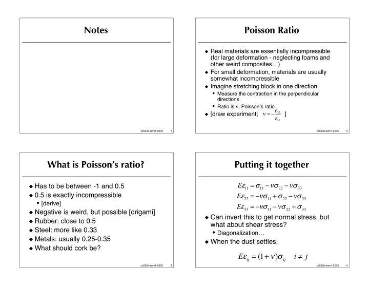
Notes Poisson Ratio � Real materials are essentially incompressible (for large deformation - neglecting foams and other weird composites…) � For small deformation, materials are usually somewhat incompressible � Imagine stretching block in one direction • Measure the contraction in the perpendicular directions • Ratio is � , Poisson � s ratio � = � � 22 � [draw experiment; ] � 11 cs533d-term1-2005 1 cs533d-term1-2005 2 What is Poisson’s ratio? Putting it together E � 11 = � 11 � �� 22 � �� 33 � Has to be between -1 and 0.5 E � 22 = � �� 11 + � 22 � �� 33 � 0.5 is exactly incompressible • [derive] E � 33 = � �� 11 � �� 22 + � 33 � Negative is weird, but possible [origami] � Can invert this to get normal stress, but � Rubber: close to 0.5 what about shear stress? � Steel: more like 0.33 • Diagonalization… � Metals: usually 0.25-0.35 � When the dust settles, � What should cork be? E � ij = (1 + � ) � ij i � j cs533d-term1-2005 3 cs533d-term1-2005 4

Inverting… Linear elasticity � � � � Putting it together and assuming constant 1 � = E � 1 + � I + 1 � 1 � � ( ) 1 � 2 � ( ) coefficients, simplifies to 1 + � � � � ˙ v = f body + � � � kk + 2 µ � � � � For convenience, relabel these ( ) = f body + � � � � x + µ � � � x + �� � x expressions E � � = • � and µ are called ( ) 1 � 2 � ( ) 1 + � the Lamé � A PDE! coefficients E µ = • We � ll talk about solving it later ( ) • [incompressibility] 2 1 + � � ij = �� kk � ij + 2 µ � ij cs533d-term1-2005 5 cs533d-term1-2005 6 Rayleigh damping Problems � Linear elasticity is very nice for small � We � ll need to look at strain rate deformation • How fast object is deforming • Linear form means lots of tricks allowed for • We want a damping force that resists change speed-up, simpler to code, … in deformation � But it � s useless for large deformation, or � Just the time derivative of strain even zero deformation but large rotation � For Rayleigh damping of linear elasticity • (without hacks) • Cauchy strain � s simplification sees large rotation as deformation… damp = � ˙ � ij � kk � ij + 2 � ˙ � � Thus we need to go back to Green strain ij cs533d-term1-2005 7 cs533d-term1-2005 8

(Almost) Linear Elasticity 2D Elasticity � Let � s simplify life before starting numerical � Use the same constitutive model as before, methods but with Green strain tensor � The world isn � t 2D of course, but want to track � This is the simplest general-purpose only deformation in the plane elasticity model � Have to model why � Animation probably doesn � t need anything • Plane strain: very thick material, � 3• =0 more complicated [explain, derive � 3• ] • Except perhaps for dealing with • Plane stress: very thin material, � 3• =0 [explain, derive � 3• and new law, note change in incompressible materials incompressibility singularity] cs533d-term1-2005 9 cs533d-term1-2005 10 Finite Volume Method Finite Element Method � Simplest approach: finite volumes � #1 most popular method for elasticity problems (and many others too) • We picked arbitrary control volumes before � FEM originally began with simple idea: • Now pick fractions of triangles from a triangle mesh • Can solve idealized problems (e.g. that strain is constant over a � Split each triangle into 3 parts, one for each corner triangle) � E.g. Voronoi regions • Call one of these problems an element � Be consistent with mass! • Can stick together elements to get better approximation • Assume A is constant in each triangle (piecewise � Since then has evolved into a rigourous mathematical linear deformation) algorithm, a general purpose black-box method • [work out] • Well, almost black-box… • Note that exact choice of control volumes not critical - constant times normal integrates to zero cs533d-term1-2005 11 cs533d-term1-2005 12

Modern Approach Weak Momentum Equation � Galerkin framework (the most common) � Ignore time derivatives - treat acceleration � Find vector space of functions that solution (e.g. X(p)) as an independent quantity lives in • We discretize space first, then use “method of • E.g. bounded weak 1st derivative: H 1 lines”: plug in any time integrator � Say the PDE is L[X]=0 everywhere (“strong”) [ ] = � ˙ � The “weak” statement is � Y(p)L[X(p)]dp=0 X � f body � � � � ˙ L X for every Y in vector space � Issue: L might involve second derivatives ( ) � � [ ] = Y � ˙ X � f body � � � � ˙ Y L X • E.g. one for strain, then one for div sigma � � • So L, and the strong form, difficult to define for H 1 � � � = Y � ˙ ˙ � � Y � � � X Yf body � Integration by parts saves the day � � � � � � = Y � ˙ ˙ � + � � Y X Yf body � � � cs533d-term1-2005 13 cs533d-term1-2005 14 Making it finite Linear Triangle Elements � The Galerkin FEM just takes the weak equation, � Simplest choice and restricts the vector space to a finite- � Take basis { � i } where dimensional one � i (p)=1 at p i and 0 at all the other p j � s • E.g. Continuous piecewise linear - constant gradient • It � s a “hat” function over each triangle in mesh, just like we used for Finite � Then X(p)= � i x i � i (p) is the continuous piecewise linear Volume Method function that interpolates particle positions � This means instead of infinitely many test � Similarly interpolate velocity and acceleration functions Y to consider, we only need to check a � Plug this choice of X and an arbitrary Y= � j (for any j) into finite basis the weak form of the equation � The method is defined by the basis � Get a system of equations (3 eq. for each j) • Very general: plug in whatever you want - polynomials, splines, wavelets, RBF � s, … cs533d-term1-2005 15 cs533d-term1-2005 16

The equations � � � � � j � ˙ i � i � � j f body + � � � j = 0 x ˙ i � � � � � � � �� j � i ˙ = � j f body � � � � j ˙ x i i � � � •Note that � j is zero on all but the triangles surrounding j, so integrals simplify •Also: naturally split integration into separate triangles cs533d-term1-2005 17