Notes Modern FEM Galerkin framework (the most common) Assignment 2 - - PowerPoint PPT Presentation

1 cs533d-term1-2005

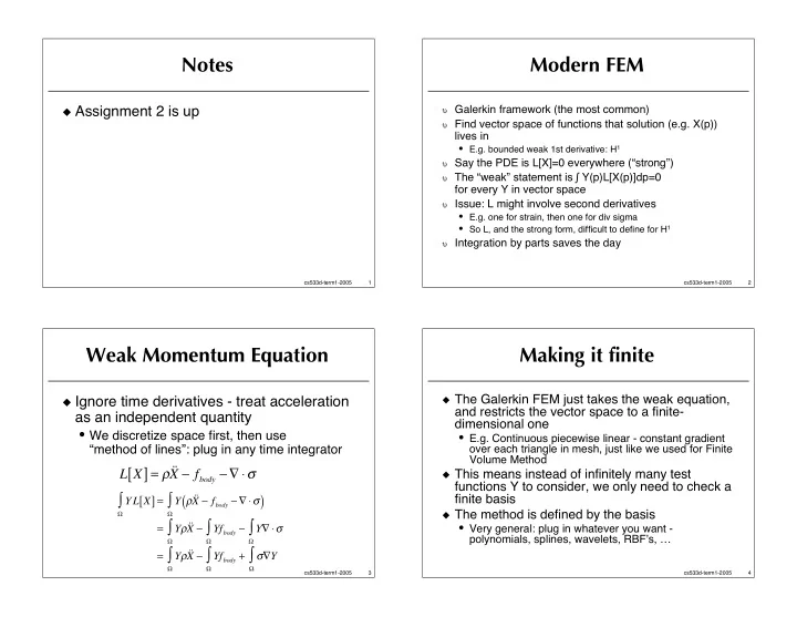
Notes

Assignment 2 is up

2 cs533d-term1-2005

Modern FEM

Galerkin framework (the most common) Find vector space of functions that solution (e.g. X(p))

lives in

• E.g. bounded weak 1st derivative: H1

Say the PDE is L[X]=0 everywhere (“strong”) The “weak” statement is Y(p)L[X(p)]dp=0

for every Y in vector space

Issue: L might involve second derivatives

• E.g. one for strain, then one for div sigma
• So L, and the strong form, difficult to define for H1

Integration by parts saves the day

3 cs533d-term1-2005

Weak Momentum Equation

Ignore time derivatives - treat acceleration

as an independent quantity

• We discretize space first, then use

“method of lines”: plug in any time integrator

L X

[ ] = ˙

˙ X fbody

Y L X

[ ]

• =

Y ˙ ˙ X fbody

( )

• =

Y˙ ˙ X

• Yfbody
• Y
• =

Y˙ ˙ X

• Yfbody
• +

Y

• 4

cs533d-term1-2005

Making it finite

The Galerkin FEM just takes the weak equation,

and restricts the vector space to a finite- dimensional one

• E.g. Continuous piecewise linear - constant gradient
• ver each triangle in mesh, just like we used for Finite

Volume Method

This means instead of infinitely many test

functions Y to consider, we only need to check a finite basis

The method is defined by the basis

• Very general: plug in whatever you want -

polynomials, splines, wavelets, RBFs, …

5 cs533d-term1-2005

Linear Triangle Elements

Simplest choice Take basis {i} where

i(p)=1 at pi and 0 at all the other pjs

• Its a “hat” function

Then X(p)=i xii(p) is the continuous piecewise linear

function that interpolates particle positions

Similarly interpolate velocity and acceleration Plug this choice of X and an arbitrary Y= j (for any j) into

the weak form of the equation

Get a system of equations (3 eq. for each j)

6 cs533d-term1-2005

The equations

j ˙ ˙ x

ii i

• j fbody
• +

j

• = 0

ji˙ ˙ x

i

• i
• =

j fbody

• j
• Note that j is zero on all but the triangles

surrounding j, so integrals simplify

• Also: naturally split integration into separate

triangles

7 cs533d-term1-2005

Change in momentum term

Let Then the first term is just Let M=[mij]: then first term is M is called the mass matrix

• Obviously symmetric (actually SPD)
• Not diagonal!

Note that once we have the forces (the other

integrals), we need to invert M to get accelerations mij = i j

• m ji˙

˙ x

i i

• M˙

˙ x

8 cs533d-term1-2005

Body force term

Usually just gravity: fbody=g Rather than do the integral with density all over

again, use the fact that I sum to 1

• They form a “partition of unity”
• They represent constant functions exactly - just about

necessary for convergence

Then body force term is gM1 More specifically, can just add g to the

accelerations; dont bother with integrals or mass matrix at all

9 cs533d-term1-2005

Stress term

Calculate constant strain and strain rate (so

constant stress) for each triangle separately

Note j is constant too So just take j times triangle area [derive what j is] Magic: exact same as FVM!

• In fact, proof of convergence of FVM is often (in other

settings too) proved by showing its equivalent or close to some kind of FEM

10 cs533d-term1-2005

The algorithm

Loop over triangles

• Loop over corners
• Compute integral terms
• nly need to compute M once though - its constant
• End up with row of M and a “force”

Solve Ma=f Plug this a into time integration scheme

11 cs533d-term1-2005

Lumped Mass

Inverting mass matrix unsatisfactory

• For particles and FVM, each particle had a mass, so

we just did a division

• Here mass is spread out, need to do a big linear solve
• even for explicit time stepping

Idea of lumping: replace M with the “lumped

mass matrix”

• A diagonal matrix with the same row sums
• Inverting diagonal matrix is just divisions - so diagonal

entries of lumped mass matrix are the particle masses

• Equivalent to FVM with centroid-based volumes

12 cs533d-term1-2005

Consistent vs. Lumped

Original mass matrix called “consistent” Turns out its strongly diagonal dominant (fairly

easy to solve)

Multiplying by mass matrix = smoothing Inverting mass matrix = sharpening Rule of thumb:

• Implicit time stepping - use consistent M

(counteract over-smoothing, solving system anyways)

• Explicit time stepping - use lumped M

(avoid solving systems, dont need extra sharpening)

13 cs533d-term1-2005

Locking

Simple linear basis actually has a major problem:

locking

• But graphics people still use them all the time…

Notion of numerical stiffness

• Instead of thinking of numerical method as just getting

an approximate solution to a real problem,

• Think of numerical method as exactly solving a

problem thats nearby

• For elasticity, were exactly solving the equations for a

material with slightly different (and not quite homogeneous/isotropic) stiffness

Locking comes up when numerical stiffness is

MUCH higher than real stiffness

14 cs533d-term1-2005

Locking and linear elements

Look at nearly incompressible materials Can a linear triangle mesh deform incompressibly?

• [derive problem]

Then linear elements will resist far too much: numerical

stiffness much too high

Numerical material “locks” FEM isnt really a black box! Solutions:

• Dont do incompressibility
• Use other sorts of elements (quads, higher order)
• …

15 cs533d-term1-2005

Quadrature

Formulas for linear triangle elements and constant

density simple to work out

Formulas for subdivision surfaces (or high-order

polynomials, or splines, or wavelets…) and varying density are NASTY

Instead use “quadrature”

• I.e. numerical approximation to integrals

Generalizations of midpoint rule

• E.g. Gaussian quadrature (for intervals, triangles, tets) or tensor

products (for quads, hexes)

Make sure to match order of accuracy [or not]

16 cs533d-term1-2005

Accuracy

At least for SPD linear problems (e.g.

linear elasticity) FEM selects function from finite space that is “closest” to solution

• Measured in a least-squares, energy-norm

sense

Thus its all about how well you can

approximate functions with the finite space you chose

• Linear or bilinear elements: O(h2)
• Higher order polynomials, splines, etc.: better

17 cs533d-term1-2005

Hyper-elasticity

Another common way to look at elasticity

• Useful for handling weird nonlinear compressibility laws, for

reduced dimension models, and more

Instead of defining stress, define an elastic potential

energy

• Strain energy density W=W(A)
• W=0 for no deformation, W>0 for deformation
• Total potential energy is integral of W over object

This is called hyper-elasticity or Green elasticity For most (the ones that make sense)

stress-strain relationships can define W

• E.g. linear relationship: W=:=trace(T)

18 cs533d-term1-2005

Variational Derivatives

Force is the negative gradient of potential

• Just like gravity

What does this mean for a continuum?

• W=W(X/p), how do you do -d/dX?

Variational derivative:

• So variational derivative is
• •W/A
• And f=•W/A
• Then stress is W/A

Easy way to do reduced

dimensional objects (cloth etc.)

Wtotal X + Y

[ ] =

W X p + Y p

• W X

p

• + W

A Y p

• = Wtotal +

W A Y p

• = Wtotal

Y W A

• 19

cs533d-term1-2005

Numerics

Simpler approach: find discrete Wtotal as a sum

• f Ws for each element
• Evaluate just like FEM, or any way you want

Take gradient w.r.t. positions {xi}

• Ends up being a Galerkin method

Also note that an implicit method might need

Jacobian = negative Hessian of energy

• Must be symmetric, and at least near stable

configurations must be negative definite