Noise " ? " " Remove Additive Erkut Erdem ! Dept. - - PowerPoint PPT Presentation

SLIDE 1

BIL 717! Image Processing!

"

Erkut Erdem!

• Dept. of Computer Engineering!

Hacettepe University! ! "

Sparse Coding

"

Acknowledgement: The slides are adapted from the ones prepared by M. Elad."

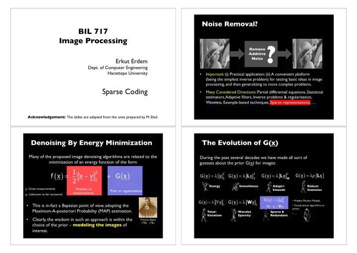
Noise Removal?"

Remove Additive Noise"?"

• Important: (i) Practical application; (ii) A convenient platform

(being the simplest inverse problem) for testing basic ideas in image processing, and then generalizing to more complex problems."

• Many Considered Directions: Partial differential equations, Statistical

estimators, Adaptive filters, Inverse problems & regularization, Wavelets, Example-based techniques, Sparse representations, …"

Relation to measurements"

Denoising By Energy Minimization "

Thomas Bayes 1702 - 1761"

Prior or regularization"

y : Given measurements " x : Unknown to be recovered"

( ) ( )

2 2

1 f x x y G x 2 = − +

Many of the proposed image denoising algorithms are related to the minimization of an energy function of the form"

• This is in-fact a Bayesian point of view, adopting the

Maximum-A-posteriori Probability (MAP) estimation."

• Clearly, the wisdom in such an approach is within the

choice of the prior – modeling the images of

• interest. "

The Evolution of G(x)"

During the past several decades we have made all sort of guesses about the prior G(x) for images: "

• Hidden Markov Models,"
• Compression algorithms as

priors, "

• …"

( )

2 2

G x x = λ

Energy"

( )

2 2

G x x = λ L

Smoothness"

( )

2

G x x = λ

W

L

Adapt+ Smooth"

( ) { }

G x x = λρ L

Robust Statistics"

( )

1

G x x = λ ∇

Total- Variation"

( )

1

G x x = λ W

Wavelet Sparsity"

( )

G x = λ α

Sparse & Redundant" α = D x for

SLIDE 2

5

Sparse Modeling of Signals "

M M

K N

D

A fixed Dictionary"

• Every column in !

D (dictionary) is ! a prototype signal (atom)."

• The vector α is

generated randomly with few (say L) non-zeros at random locations and with random

• values. "

A sparse & random vector"

=

α

x

N

• We shall refer to

this model as

Sparseland!

Interesting Model:"

• Simple: Every generated signal is

built as a linear combination of few atoms from our dictionary D"

• Rich: A general model: the
• btained signals are a union of

many low-dimensional Gaussians."

• Familiar: We have been using

this model in other context for a while now (wavelet, JPEG, …)."

Sparseland Signals are Special"

Multiply by D

α D = x

M

α

Sparse & Redundant Rep. Modeling?"

x where is sparse = α α D

Our signal ! model is thus: "

• 1

+1 1

( )

p

f x x = x

Sparse & Redundant Rep. Modeling?"

k p p j p j 1 =

α = α

∑

1 1

α

2 2

α

p p

p 1 α <

p

p p

→ α

x where is sparse = α α D

Our signal ! model is thus: "

SLIDE 3

• 1

+1 1

( )

p

f x x = x

Sparse & Redundant Rep. Modeling?"

1 1

α

2 2

α

p p

p 1 α <

p

p p

→ α

As p ! 0 we get a count!

• f the non-zeros

in the vector"

α

x where is sparse = α α D

Our signal ! model is thus: "

x where L = α α ≤ D

• L0 norm effectively

counts the number of non-zeros in α. "

• The vector α is the

representation (sparse/redundant)

• f the desired

signal x."

• The core idea: while few (L out of K) atoms can be merged

to form the true signal, the noise cannot be fitted well. Thus, we

• btain an effective projection of the noise onto a very

low-dimensional space, thus getting denoising effect. "

α = ≤ α − α = α

α

ˆ x ˆ L . t . s y 2 1 min arg ˆ

2 2

D D

Dα-y = -

Back to Our MAP Energy Function "

x

Wait! There are Some Issues "

• Numerical Problems: How should we solve or approximate the

solution of the problem"

"

" " " " " or " "

• r ?"

"

• Theoretical Problems: Is there a unique sparse representation? If we

are to approximate the solution somehow, how close will we get? "

"

• Practical Problems: What dictionary D should we use, such that all

this leads to effective denoising? Will all this work in applications?"

"

L . t . s y min

2 2

≤ α − α

α

D

2 2 2

y . t . s min ε ≤ − α α

α

D

2 2

min y

α

λ α + α − D

To Summarize So Far …"

Use a model for signals/images based

• n sparse and

redundant representations" What can we do? " Image denoising (and many other problems in image processing) requires a model for the desired image" Great! No?" There are some issues: " 1. Theoretical" 2. How to approximate?" 3. What about D?"

SLIDE 4

Known "

Lets Start with the Noiseless Problem"

ArgMin s.t. x ˆ

α

α = α = α D

We aim to find the signal’s representation: " Suppose we build a signal by the relation"

=

x α= D

ˆ α = α

Why should we necessarily get ?" " It might happen that eventually ."

ˆ α < α

Uniqueness"

Matrix “Spark”"

Rank = 4" Spark = 3"

⎡ ⎤ ⎢ ⎥ ⎢ ⎥ ⎢ ⎥ ⎢ ⎥ ⎣ ⎦ 1 1 1 1 1 1

Example:"

Donoho & E. (‘02) "

Definition: Given a matrix D, σ =Spark{D} is the smallest " " number of columns that are linearly dependent. "

* "In tensor decomposition, Kruskal defined something similar already in 1989."

*"

Uniqueness Rule"

ArgMin s.t. x ˆ

α

α = α = α D

Suppose this problem has been solved somehow" This result implies that if generates signals using “sparse enough” α, the solution of the above will find it exactly."

M

If we found a representation that satisfy "

"

"

Then necessarily it is unique (the sparsest)."

ˆ 2 σ α <

Uniqueness"

" Donoho & E. (‘02) "

Our Goal "

This is a combinatorial problem, proven to be NP-Hard! " Here is a recipe for solving this problem:" Set L=1 " Gather all the supports {Si}i

• f cardinality L "

LS error 2 ?"

2 2 2

y . t . s min ε ≤ − α α

α

D

Solve the LS problem " " for each support " ( )

i 2 2

S p sup . t . s y min = α − α

α

D

Set L=L+1 " There are (K) such supports"

L"

Yes" No"

Done"

Assume: K=1000, L=10 (known!), 1 nano-sec per each LS" We shall need ~8e+6 years to solve this problem !!!!!"

SLIDE 5

Lets Approximate "

2 2 2

y . t . s min ε ≤ − α α

α

D

Greedy methods" Build the solution one non-zero element at a time" Relaxation methods" Smooth the L0 and use continuous optimization techniques"

Relaxation – The Basis Pursuit (BP)"

ε ≤ − α α

α 2

y . t . s Min D Instead of solving" ε ≤ − α α

α 2 1

y . t . s Min D Solve Instead"

• This is known as the Basis-Pursuit (BP) [Chen, Donoho & Saunders (’95)]."
• The newly defined problem is convex (quad. programming)."
• Very efficient solvers can be deployed:"

" Interior point methods [Chen, Donoho, & Saunders (‘95)] [Kim, Koh, Lustig, Boyd, & D.

Gorinevsky (`07)]."

" Sequential shrinkage for union of ortho-bases [Bruce et.al. (‘98)]." " Iterative shrinkage [Figuerido & Nowak (‘03)] [Daubechies, Defrise, & De-Mole (‘04)]

[E. (‘05)] [E., Matalon, & Zibulevsky (‘06)] [Beck & Teboulle (`09)] … "

Go Greedy: Matching Pursuit (MP)"

≅

• Next steps: given the previously found atoms,

find the next one to best fit the residual."

• The algorithm stops when the error is below the destination

threshold."

• The MP is one of the greedy

algorithms that finds one atom at a time [Mallat & Zhang (’93)]."

• Step 1: find the one atom that best

matches the signal. "

• The Orthogonal MP (OMP) is an improved version that re-evaluates the

coefficients by Least-Squares after each round."

2

y − α D

21"

Pursuit Algorithms"

There are various algorithms designed for approximating the solution

• f this problem: "

2 2 2

y . t . s min ε ≤ − α α

α

D

• Greedy Algorithms: Matching Pursuit, Orthogonal Matching Pursuit (OMP),

Least-Squares-OMP , Weak Matching Pursuit, Block Matching Pursuit [1993- today]."

• Relaxation Algorithms: Basis Pursuit (a.k.a. LASSO), Dnatzig Selector &

numerical ways to handle them [1995-today]."

• Hybrid Algorithms: StOMP

, CoSaMP , Subspace Pursuit, Iterative Hard- Thresholding [2007-today]."

• …"

SLIDE 6

22"

Pursuit Algorithms"

There are various algorithms designed for approximating the solution

• f this problem: "

2 2 2

y . t . s min ε ≤ − α α

α

D

• Greedy Algorithms: Matching Pursuit, Orthogonal Matching Pursuit (OMP),

Least-Squares-OMP , Weak Matching Pursuit, Block Matching Pursuit [1993- today]."

• Relaxation Algorithms: Basis Pursuit (a.k.a. LASSO), Dnatzig Selector &

numerical ways to handle them [1995-today]."

• Hybrid Algorithms: StOMP

, CoSaMP , Subspace Pursuit, Iterative Hard- Thresholding [2007-today]."

• …"

Why should they work" ?"

The Mutual Coherence"

• The Mutual Coherence μ is the largest off-diagonal

entry in absolute value." DT"

="

D" DTD"

• Compute"
• The Mutual Coherence is a property of the dictionary (just

like the “Spark”). In fact, the following relation can be shown: "

σ ≥ + µ 1 1

Assume normalized columns"

BP and MP Equivalence (No Noise)"

ArgMin s.t. x ˆ

α

α = α = α D

BP and MP Equivalence (No Noise)"

Given a signal x with a representation ," assuming that , BP and MP " are guaranteed to find the sparsest solution. " "

x = α D ( )

α < + µ 0.5 1 1

Donoho & E. (‘02) " Gribonval & Nielsen (‘03)" Tropp (‘03) " Temlyakov (‘03)" "

Equivalence"

• MP and BP are different in general (hard to say which is better)."
• The above result corresponds to the worst-case, and as such, it is too

pessimistic."

• Average performance results are available too, showing much better

bounds [Donoho (`04)] [Candes et.al. (‘04)] [Tanner et.al. (‘05)] !

[E. (‘06)] [Tropp et.al. (‘06)] … [Candes et. al. (‘09)]. "

SLIDE 7

BP Stability for the Noisy Case "

2 1 2

min y

α

λ α + α − D

BP Stability for the Noisy Case "

• For σ=0 we get a weaker version of the previous result."
• This result is the oracle’s error, multuiplied by C· logK."
• Similar results exist for other pursuit algorithms (Dantzig Selector, Orthogonal

Matching Pursuit, CoSaMP , Subspace Pursuit, …)"

Given a signal with a representation" satisfying and a white Gaussian " noise , BP will show stability, i.e., " α < µ 1 / 3

Ben-Haim, Eldar & E. (‘09)"

Stability"

v y + α = D

2 2 BP 2

Const( ) logK ˆ α − α < λ ⋅ ⋅ α ⋅ σ

( )

2

v ~ N 0,σ I

* With very high " probability"

*"

To Summarize So Far …

Use a model for signals/images based on sparse and redundant representations

What do we do?

Image denoising (and many other problems in image processing) requires a model for the desired image We have seen that there are approximation methods to find the sparsest solution, and there are theoretical results that guarantee their success.

Problems? What next?

The Dictionary D should be found somehow !!!

31" α = ε ≤ − α α = α

α

ˆ x ˆ and y 2 1 . t . s min arg ˆ

2 2 2

D D

What Should D Be? "

Our Assumption: Good-behaved Images have a sparse representation" D should be chosen such that it sparsifies the representations" The approach we will take for building D is training it, based on Learning from ! Image Examples " One approach to choose D is from a known set of transforms (Steerable wavelet, Curvelet, Contourlets, Bandlets, Shearlets …)"

SLIDE 8

32"

Each example is a linear combination

• f atoms from D"

Measure of Quality for D"

D"

"

X" A"

Each example has a sparse representation with no more than L atoms"

L , j . t . s x Min

j P 1 j 2 2 j j ,

≤ α ∀ − α

∑

=

D

A D

[Field & Olshausen (‘96)]" [Engan et. al. (‘99)]" [Lewicki & Sejnowski (‘00)]" [Cotter et. al. (‘03)]" [Gribonval et. al. (‘04)]" [Aharon, E. & Bruckstein (‘04)] [Aharon, E. & Bruckstein (‘05)]" "

33"

K–Means For Clustering "

D"

Initialize D" Sparse Coding"

Nearest Neighbor"

Dictionary Update"

Column-by-Column by Mean computation over the relevant examples"

X

T"

Clustering: An extreme sparse representation "

34"

The K–SVD Algorithm – General "

D"

Initialize D" Sparse Coding"

Use Matching Pursuit"

Dictionary Update"

Column-by-Column by SVD computation over the relevant examples"

[Aharon, E. & Bruckstein (‘04,‘05)]"

X

T"

35"

K–SVD: Sparse Coding Stage"

D"

X

T"

L , j . t . s x Min

p p j P 1 j 2 2 j j

≤ α ∀ ∑ − α

=

D

A

D is known! For the jth item we solve " L . t . s x Min

p p 2 2 j

≤ α − α

α

D Solved by A Pursuit Algorithm"

SLIDE 9

K–SVD: Dictionary Update Stage"

D"

Refer only to the examples that use the column dk" ? dk = Fixing all A and D apart from the kth column, and seek both dk and the kth column in A to better fit the residual!" We should solve:"

2 F T k k , d

d Min

k k

E − α

α

K–SVD: Dictionary Update Stage"

D"

Refer only to the examples that use the column dk" ? dk = Fixing all A and D apart from the kth column, and seek both dk and the kth column in A to better fit the residual!" We should solve:"

2 F T k k , d

d Min

k k

E − α

α

S V D "

To Summarize So Far …

Use a model for signals/images based on sparse and redundant representations

What do we do?

Image denoising (and many other problems in image processing) requires a model for the desired image We have seen that there are approximation methods to find the sparsest solution, and there are theoretical results that guarantee their success.

Problems? What next?

Will it all work in applications?

Our prior"

Extracts a patch in the ij location"

• The K-SVD algorithm is reasonable for low-

dimension signals (N in the range 10-400).! As N grows, the complexity and the memory requirements of the K-SVD become prohibitive. "

• So, how should large images be handled?"

L . t . s x y x 2 1 ArgMin x ˆ

ij ij 2 2 ij ij 2 2 } { , x

ij ij

≤ α ∑ α − µ + − =

α

D R

From Local to Global Treatment"

D"

N"

k"

• The solution: Force shift-invariant sparsity - on each patch of size !

N-by-N (N=8) in the image, including overlaps. "

SLIDE 10

Option 1:"

• Use a database of images,"
• We tried that, and it works fine (~0.5-1dB

below the state-of-the-art). " Option 2: "

• Use the corrupted image itself !! "
• Simply sweep through all patches of size

N-by-N (overlapping blocks), "

• Image of size 10002 pixels ~106

examples to use – more than enough."

• This works much better!"

What Data to Train On?"

Complexity of this algorithm: O(N2×K×L×Iterations) per pixel. For N=8, L=1, K=256, and 10 iterations, we need 160,000 (!!) operations per pixel. "

K-SVD"

L . t . s x y x ArgMin x ˆ

ij ij 2 2 ij ij 2 2 2 1 , } { , x

ij ij

≤ α α − µ + − =

∑

α

D R

D

x=y and D known"

L . t . s x Min

2 2 ij ij

≤ α α − = α

α

D R Compute αij per patch "

" "

" using the matching pursuit"

x and αij known"

∑ α −

α ij 2 2 ijx

Min D R Compute D to minimize " " " using SVD, updating one column at a time"

D and αij known"

⎥ ⎥ ⎦ ⎤ ⎢ ⎢ ⎣ ⎡ α µ + ⎥ ⎥ ⎦ ⎤ ⎢ ⎢ ⎣ ⎡ µ + =

∑ ∑

− ij ij T ij 1 ij ij T ij

y I x D R R R

Compute x by" " " which is a simple averaging of shifted patches"

K-SVD Image Denoising"

D?"

Initial dictionary (overcomplete DCT) 64×256"

Image Denoising (Gray) [E. & Aharon (‘06)]"

Source" Result 30.829dB" The obtained dictionary after ! 10 iterations" Noisy image "

20 = σ

Initial dictionary (overcomplete DCT) 64×256"

Image Denoising (Gray) [E. & Aharon (‘06)]"

Source" Result 30.829dB" The obtained dictionary after ! 10 iterations" Noisy image "

20 = σ

• The results of the K-SVD algorithm compete favorably

with the state-of-the-art. "

• In a recent work that extended this algorithm to use

joint sparse representation on the patches, the best published denoising performance are obtained [Mairal,

Bach, Ponce, Sapiro & Zisserman (‘09)]."

SLIDE 11

Denoising (Color) [Mairal, E. & Sapiro (‘08)]"

• When turning to handle color images, the main

difficulty is in defining the relation between the color layers – R, G, and B. "

• The solution with the above algorithm is simple

– consider 3D patches or 8-by-8 with ! the 3 color layers, and the dictionary! will detect the proper relations. "

Denoising (Color) [Mairal, E. & Sapiro (‘08)]"

Original Noisy (20.43dB) Result (30.75dB)"

Denoising (Color) [Mairal, E. & Sapiro (‘08)]"

Original Noisy (12.77dB) Result (29.87dB)" The K-SVD algorithm leads to state-of-the-art denoising results, giving ~1dB better results compared to [Mcauley et. al. (‘06)] ! which implements a learned MRF model (Field-of-Experts)"

Video Denoising [Protter & E. (‘09)]"

When turning to handle video, one could improve

• ver the previous scheme in three important ways:"
• 1. Propagate the dictionary from one frame to

another, and thus reduce the number of iterations; "

• 2. Use 3D patches that handle the motion

implicitly; and"

• 3. Motion estimation and

compensation can and should be avoided

[Buades, Col, and Morel (‘06)]. "

SLIDE 12

Original Noisy (=25) Denoised (PSNR=27.62)" Original Noisy (=15) Denoised (PSNR=29.98)"

Video Denoising [Protter & E. (‘09)]"

Original Noisy (=25) Denoised (PSNR=27.62)" Original Noisy (=15) Denoised (PSNR=29.98)"

Video Denoising [Protter & E. (‘09)]"

The K-SVD algorithm leads to state-of-the-art video denoising results, giving ~0.5dB better results on average compared to [Boades, Coll & Morel (‘05)] and comparable to [Rusanovskyy, Dabov, & Egiazarian (‘06)]"

Low-Dosage Tomography [Shtok, Zibulevsky & E. (‘10)]"

• In Computer-Tomography (CT) reconstruction, an image is

recovered from a set of its projections. "

"

• In medicine, CT projections are obtained by X-ray, and it

typically requires a high dosage of radiation in order to

• btain a good quality reconstruction. "

"

• A lower-dosage projection implies a stronger noise

(Poisson distributed) in data to work with. "

• Armed with sparse and redundant representation

modeling, we can denoise the data and the final reconstruction … enabling CT with lower dosage."

Low-Dosage Tomography [Shtok, Zibulevsky & E. (‘10)]"

Original" FBP result with high dosage" " PSNR=24.63dB" FBP result with low dosage (one fifth)" " PSNR=22.31dB" Denoising of the sinogram and post- processing (another denoising stage) of the reconstruction" " PSNR=26.06dB"

SLIDE 13

Image Inpainting – The Basics "

• Assume: the signal x has been created

by x=D0 with very sparse 0. "

• Missing values in x imply

missing rows in this linear

• system. "
• By removing these rows, we get ."
• Now solve"

"

• If 0 was sparse enough, it will be the solution of the above

problem! Thus, computing D0 recovers x perfectly."

x α = D

="

x α = D  

Min s.t. x

α

α = α D  

Side Note: Compressed-Sensing"

• Compressed Sensing is leaning on the very same principal, leading to

alternative sampling theorems."

=

• Assume: the signal x has been created by x=D0 with very sparse 0. "
• Multiply this set of equations by the matrix Q which reduces the

number of rows."

• The new, smaller, system of equations is"

x x α = α = QD Q D  

×

• If 0 was sparse enough, it will be the sparsest solution of the new

system, thus, computing D0 recovers x perfectly."

• Compressed sensing focuses on conditions for this to happen,

guaranteeing such recovery."

Result" Experiments lead to state-of-the-art inpainting results." Original 80% missing"

Inpainting [Mairal, E. & Sapiro (‘08)]"

Experiments lead to state-of-the-art inpainting results."

Inpainting [Mairal, E. & Sapiro (‘08)]"

Original 80% missing" Result"

SLIDE 14

Experiments lead to state-of-the-art inpainting results."

Inpainting [Mairal, E. & Sapiro (‘08)]" Inpainting [Mairal, E. & Sapiro (‘08)]"

Original 80% missing " " Result"

The same can be done for video, very much like the denoising treatment: (i) 3D patches, (ii) no need to compute the dictionary from scratch for each frame, and (iii) no need for explicit motion estimation"

Demosaicing [Mairal, E. & Sapiro (‘08)]"

• Today’s cameras are sensing only one

color per pixel, leaving the rest for interpolated."

• Generalizing the inpainting scheme to

handle demosaicing is tricky because

• f the possibility to learn the mosaic

pattern within the dictionary."

• In order to avoid “over-fitting”, we handle

the demosaicing problem while forcing strong sparsity and applying only few

• iterations. "

Experiments lead to state-of-the-art demosaicing results, giving ~0.2dB better results on average, compared to [Chang & Chan (‘06)]"

Demosaicing [Mairal, E. & Sapiro (‘08)]"

SLIDE 15

Image Compression [Bryt and E. (‘08)]"

• The problem: Compressing photo-ID images."
• General purpose methods (JPEG, JPEG2000) !

do not take into account the specific family. "

• By adapting to the image-content (PCA/K-SVD),

better results could be obtained."

• For these techniques to operate well, train

dictionaries locally (per patch) using a training set of images is required."

• In PCA, only the (quantized) coefficients are stored,

whereas the K-SVD requires storage of the indices as well."

• Geometric alignment of the image is very helpful

and should be done [Goldenberg, Kimmel, & E. (‘05)]. "

Image Compression"

Training set (2500 images)"

Detect main features and warp the images to a common reference (20 parameters) "

On the training set"

Divide the image into disjoint 15- by-15 patches. For each compute mean and dictionary " Per each patch find the operating parameters (number of atoms L, quantization Q) " Warp, remove the mean from each patch, sparse code using L atoms, apply Q, and dewarp"

On the test image"

69"

Image Compression Results"

Results ! for 820 Bytes per each file"

11.99" 10.83" 10.93" 10.49" 8.92" 8.71" 8.81" 7.89" 8.61" 5.56" 4.82" 5.58"

Original" JPEG" JPEG-2000" Local-PCA" K-SVD"

70"

Results ! for 550 Bytes per each file"

15.81" 14.67" 15.30" 13.89" 12.41" 12.57" 10.66" 9.44" 10.27" 6.60" 5.49" 6.36"

Image Compression Results"

Original" JPEG" JPEG-2000" Local-PCA" K-SVD"

SLIDE 16

71"

Results ! for 400 Bytes per each file"

18.62" 16.12" 16.81" 12.30" 11.38" 12.54" 7.61" 6.31" 7.20"

?" ?" ?"

Image Compression Results"

Original" JPEG" JPEG-2000" Local-PCA" K-SVD"

72"

550 bytes ! K-SVD results with and without deblocking"

Deblocking the Results [Bryt and E. (`09)]"

K-SVD (6.60)" K-SVD (11.67)" K-SVD (6.45)" K-SVD (5.49)" Deblock (6.24)" Deblock (11.32)" Deblock (6.03)" Deblock (5.27)"

73"

Super-Resolution [Zeyde, Protter, & E. (‘11)] "

• Given a low-resolution image, we desire to enlarge it while

producing a sharp looking result. This problem is referred to as “Single-Image Super-Resolution”."

• Image scale-up using bicubic interpolation is far from being

satisfactory for this task. "

• Recently, a sparse and redundant representation technique

was proposed [Yang, Wright, Huang, and Ma (’08)] for solving this problem, by training a coupled-dictionaries for the low- and high res. images. "

• We extended and improved their algorithms and results."

SR Result" PSNR=16.95dB" Bicubic interpolation PSNR=14.68dB" 75"

Super-Resolution – Results (1)"

The training image: 717×717 pixels, providing a set of 54,289 training patch- pairs."

SLIDE 17

Ideal Image" Given Image" SR Result" PSNR=16.95dB" Bicubic interpolation PSNR=14.68dB" 76"

Super-Resolution – Results (1)"

Given image"

Scaled-Up (factor 2:1) using the proposed algorithm, PSNR=29.32dB (3.32dB improvement over bicubic)"

77"

Super-Resolution – Results (2)"

The Original Bicubic Interpolation SR result "

78"

Super-Resolution – Results (2)"

The Original Bicubic Interpolation SR result "

79"

Super-Resolution – Results (2)"