My next 10 years Galaxy Survey: HETDEX CMB Polarization: LiteBIRD - - PowerPoint PPT Presentation

My next 10 years

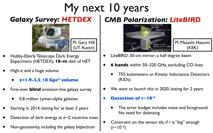
• Hobby-Eberly Telescope Dark Energy

Experiment (HETDEX); 10-m dish of HET

• High-z; and a huge volume
• z=1.9–3.5; 10 Gpc3 volume
• First-ever blind emission-line galaxy survey
• 0.8 million Lyman-alpha galaxies
• Starting in 2014, lasting for at least 3 years
• Detection of dark energy at z~2; neutrino mass
• Non-gaussianity, including the galaxy bispectrum

Galaxy Survey: HETDEX CMB Polarization: LiteBIRD

PI: Gary Hill (UT Austin) PI: Masashi Hazumi (KEK)

• LiteBIRD; 30-cm mirror; a half degree beam
• 6 bands within 50–320 GHz, excluding CO lines
• TES bolometers or Kinetic Inductance Detectors

(KIDs)

• We want to launch this in 2020, lasting for 2 years
• Detection of r~10–3
• The error budget includes noise and foreground.

No need for delensing

• Constraint on the tensor tilt, if r is “big” enough

(r~10–2)

So, my next 10 years will be...

• ...devoted to the continuation of what we have been

doing over the last few decades

• COBE -> WMAP -> Planck -> LiteBIRD
• CfA -> 2dF/SDSS -> WiggleZ/BOSS -> HETDEX/others
• “Inertial motion” = a continuation from the past
• These are important steps forward in measurements;

however, do we really want to be in inertial motion forever?

What Are the New Challenges For Early Universe Cosmologists?

Eiichiro Komatsu (Max-Planck-Institut für Astrophysik) “New Challenges for Early Universe Cosmologists,” Lorentz Center Conference, August 9, 2013

New Challenges in the Post-Planck Era

• I heard many people saying “I was disappointed by the

Planck results. Cosmology is boring now!”

• What are the challenges now? Challenges are in
• ur mind. In my point of view, the post-Planck world

provides new opportunities, because...

New Opportunities in the Post-Planck Era

• An important milestone has been achieved: ns<1 is now
• discovered. And...

New Opportunities in the Post-Planck Era

July 11, 2013

ns~0.96 [Mukhanov & Chibisov 1981], now observed; and the R2 inflation [Starobinsky 1980], continues to fit the data rather well

• But...

New Opportunities in the Post-Planck Era

• But... these predictions were made a long time ago.

Finally discovering ns<1 is wonderful and remarkable, but what else can younger generations contribute to this field? Not much, really...

• Similarly:

New Opportunities in the Post-Planck Era

• Similarly: imagine that fNL was discovered in the

Planck data. That would be a remarkable achievement, revolutionizing the field of inflation.

• However, a lot of fundamental work have already been

done on fNL, and frankly there would not be too much left for younger generations to chew on, even if it was

• detected. Therefore...

New Opportunities in the Post-Planck Era

• Therefore... younger generations should be glad that

the Planck data continue to support vanilla single-field inflation models because this means that all of us, junior

• r senior, are back on the same starting line!

You don’t have to read too many papers on fNL!

Advice from Hayashi

• Chushiro Hayashi:
• “A good research area is the one that has the least

references.”

Chushiro Hayashi

(Takashi Nakamura)

“Thinking outside the box”

• Challenges are in our mind. Yes, it is difficult to

find something novel if we work on the subjects along the line of what has been done already.

• One of the challenges in our mind: worrying too much

about the observability in a short time scale.

• Just forget about the observability. If the physics is

beautiful, it is worth doing!

Learning from the past

• Slava Mukhanov:
• “I thought that it would take 1000 years to detect the

logarithmic dependence of the power spectrum.”

ns=0.960±0.007

Learning from the past

• Rashid Sunyaev:
• “I did not think that the acoustic oscillation would

ever be observed.”

Rashid Sunyaev

Learning from the past

• Jim Peebles (Annu. Rev. Astro. Astrophys. 2012):
• “I did not continue with (computation of CMB), in

part because I had trouble imagining that such tiny disturbances to the CMB could be detected...”

Jim Peebles

Learning from the past

• Yakov Zel’dovich:
• “(Speaking to Sunyaev about the Sunyaev-Zel’dovich

effect:) This is a small effect, but the physics is

• beautiful. Let’s publish it.”

Yakov Zel’dovich

An Example

• The energy density spectrum of primordial gravitational
• waves. It is usually said that it goes as 1/(frequency)2 in

the low-frequency region and is constant in the high- frequency region. ΩGW frequency ~10–16 Hz

Previous Lore

ρuniv~1/a3 ρuniv~1/a4

Previous Lore

ρuniv~1/a3 ρuniv~1/a4

Jumps in the number of radiation species

Quark-Hadron phase transition e+e– annihilation

Correct spectrum in the Standard Model

Watanabe & Komatsu (2006)

Einflation=1016 GeV CMB scale

Watanabe & Komatsu (2006)

Yes, people do ask:

• “Is this effect ever measurable?”
• And my answer is always: “I do not care.”
• The lesson we have learned from CMB experiments

is that, if experimentalists are convinced that it is worth measuring, they will get there much sooner than you’d think!

• Theorist’s job is to find something which may be

small, but is worth measuring.

A Good Working Hypothesis

• B-mode polarization will be found at the level of r~10–3
• r greater by, e.g., LiteBIRD (a Japan-led polarization

satellite mission).

• The scale-invariance of gravitational waves also

measured at, say, 10% level. Inflation is proven.

• The challenge: then what?

Some Challenging Questions

• How inflation happened?
• How inflation started; how inflation ended?
• What is inflaton?
• Do fluctuations really have the quantum origin?

How inflation happened?

• What can we measure to say anything at all about the
• rigin of inflation?
• The necessary working hypothesis: the number of e-

folds is the minimum value required to solve the horizon problem (or the flatness problem for open inflation).

How inflation happened?

• What can we measure to say anything at all about the origin
• f inflation? A few candidates:
• Curvature
• Pre-inflationary relics (e.g., bubble collision)
• Coupling of modes in the pre-inflationary phase (e.g.,

super-curvature modes in open inflation) to the

• bservable modes
• Non-Bunch-Davies initial state from quantum tunneling

[Bζ-> e–πks/(kL4kS2); Sugimura&Komatsu, to appear]

Quantum Fluctuations

• The fundamental prediction of inflation is that

fluctuations originated from quantum fluctuations.

• How can we test this?

Quantum or Classical?

The large-scale modes commute!

conjugate momentum

Quantum or Classical?

• Super-horizon modes become “classical” (in a sense of a

vanishing commutation relation).

• However, when they re-enter the horizon, they become

quantum again.

• We know that scalar perturbations did not become

quantum again; so some decoherence must have happened to scalar perturbations.

• But, how about gravitational waves?

Squeezed State from Inflation

• Inflation predicts that, on

super-horizon scales, the variance in the field value (vk) is much greater than the variance in the conjugate momentum (pk).

• The area in vk-pk remains

the same: no violation of Heisenberg’s uncertainty principle (of course).

Sub-horizon (coherent; Gaussian) Super-horizon (squeezed; still Gaussian, but elongated in

• ne direction)

Figure from Martin, Vennin & Peter (2012)

Grishchuk & Sidorov (1989;1990)

Squeezing on Super-horizon Scales

• Solution for the field (de Sitter): vk ~ (2k3)–1/2(1+ikη)e–ikη
• Conjugate momentum: pk=vk’ ~ (2k3)–1/2k2ηe–ikη
• The ratio of the variances:
• k2|vk|2/|pk|2 = |1+ikη|2/(kη)2
• -> 1 for kη->∞ [coherent state]
• -> k–2 for kη->0 [squeezed]

Squeezed State and Tests of Gaussianity

• The squeezed quantum state is statistically indistinguishable

from an ensemble of classical fluctuations

• Coherent state: localized in vk and pk, the trajectory of

the packet obeying the classical equation of motion

• Inflationary squeezed state: not localized in vk,

equivalent to having many classical trajectories

• Therefore, tests of Gaussianity treating cosmological

fluctuations as an ensemble of classical fluctuations do

• ffer a test of the squeezed state

Question

• While testing the squeezed state is not necessarily a

test of quantum fluctuations, can we test this more directly than Gaussianity tests?

• It is not clear to me how much more information we

learn about inflation by testing the squeezed state more directly, but let me proceed.

Testing Squeezed State

• Primordial gravitational waves should be in a squeezed

state (Grishchuk & Sidorov 1989;1990). If we can see individual gravitons, they look like #3: #1 #2 #3

#1: anti-bunched; sub-Poisson; <n2>–<n>2 smaller than <n> #2: un-bunched; Poisson; <n2>–<n>2 equal to <n> #3: bunched; super-Poisson; <n2>–<n>2 larger than <n> coherent state

Hanbury Brown-Twiss (HBT) Interferometry

• Imagine that we measure + or x modes of gravitational waves.

Then measure the following ratio called the “second-order coherence”:

• g(2)(τ)=<h(t)h(t+τ)h*(t)h*(t+τ)>/(<h(t)h*(t)><h(t+τ)h*(t+τ)>)

g(2)(0)>1 g(2)(0)=1 g(2)(0)<1

• Imagine that we measure + or x modes of gravitational waves.

Then measure the following ratio called the “second-order coherence”:

• g(2)(τ)=<h(t)h(t+τ)h*(t)h*(t+τ)>/(<h(t)h*(t)><h(t+τ)h*(t+τ)>)

Hanbury Brown-Twiss (HBT) Interferometry

Inflation predicts g(2)(0)≈3! (Grishchuk&Sidorov 1989) cf: chaotic light (light emitted by uncorrelated sources) gives g(2)(0)=2 Can this distinguish between the vacuum fluctuations and classical sources of GW? g(2)(0)>1 g(2)(0)=1 g(2)(0)<1

Summary

• New challenges = New opportunities. We are back on

the same starting line.

• Learning from the past: Do not pay attention to the
• bservability. If it is worth measuring it, we will get there.
• Challenging, but potentially testable, questions:
• How inflation happened? Testing quantum tunneling

models (assuming N~Nminimum)

• Are fluctuations quantum? HBT interferometry of

Gravitational waves to find a squeezed state?