
SLIDE 1
Multiple Single-Facility Location
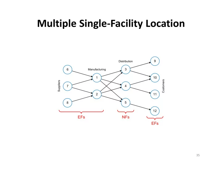
Suppliers Manufacturing Customers
10 9 11 12 3 4 5 1 2 6 7 8
Distribution
EFs EFs NFs
35
Multiple Single-Facility Location 9 Distribution 3 6 - - PowerPoint PPT Presentation
Multiple Single-Facility Location 9 Distribution 3 6 Manufacturing 1 10 Customers Suppliers 7 4 2 11 5 8 12 EFs NFs EFs 35 Best Retail Warehouse Locations 36 Optimal Number of NFs TC Transport Cost 1 2 3 4 5 6 Number
Suppliers Manufacturing Customers
10 9 11 12 3 4 5 1 2 6 7 8
Distribution
EFs EFs NFs
35
36
1 5 2 3 4 6
Transport Cost
TC Number of NFs
37
– Cost data from existing facilities can be used to fit linear estimate
– Economies of scale in production
k > 0 and β < 1
38
max
act min est act 1 act est
max , 0.62, Hand tool mfg. 0.48, Construction 0.41, Chemical processing 0.23, Medical centers fixed cost
f f p p p
f TPC TPC TPC f TPC c f TPC TPC APC f f f k APC c f k k c
β β β
β
< −
= = = + = = = + =
min max MES
constant unit production cost / min/max feasible scale / base cost/rate f f f Minimum Efficient Scale TPC f = = = =
fmin fMES f0 fmax
Production Rate (ton/yr)
TPCmin
k
TPC0
cp
TPCact ( = 0.5) TPCest Actual EF cost APCact APCest
i
39
1 4 2 6 3 5 1 2 3 4
1
x
2
x
1 2 1 2 1 1 2
max 6 8 s.t. 2 3 11 2 7 , x x x x x x x + + ≤ ≤ ≥
6 8 2 3 11 , 2 7 = = = c A b
* *
1 3 2 2 , 31 1 3 13 ′ = = x c x
1 4 2 6 3 5 1 2 3 4
2 313 1 2 1 2 1 1 2 1 2
max 6 8 s.t. 2 3 11 2 7 , , integer x x x x x x x x x + + ≤ ≤ ≥
1
[ ]
6 8 2 3 11 , 2 7 = = = c A b
2
1 313 26 31 2 303 28 30 2 31 , 3 UB LB = =
1
3 x ≤
1
4 x ≥
2
1 x ≤
2
2 x ≥
1
2 x ≤
1
3 x ≥
2
2 x ≤
2
3 x ≥
1 31 , 3 UB LB = = 1 31 , 26 3 UB LB = =
31, 26 UB LB = =
2 30 , 26 3 UB LB = = 2 30 , 30 3 2 30 30 1 3 UB LB gap = = = − < 2 30 , 28 3 UB LB = =
40
i i ij ij i N i N j M ij i N i ij ij i
∈ ∈ ∈ ∈
where fixed cost of NF at site 1,..., variable cost from to serve EF 1,..., 1, if NF established at site 0,
fraction of EF demand served from NF at site .
i ij i ij
k i N n c i j M m i y x j i = ∈ = = ∈ = = =
41
ij ij i N j M i i N ij i N i ij ij i
∈ ∈ ∈ ∈
where number of NF to establish variable cost from to serve EF 1,..., 1, if NF established at site 0,
fraction of EF demand served from NF at site .
ij i ij
p c i j M m i y x j i = = ∈ = = =
42