Motion and optical flow repeating patterns of local structure - - PDF document

9/16/2015 1

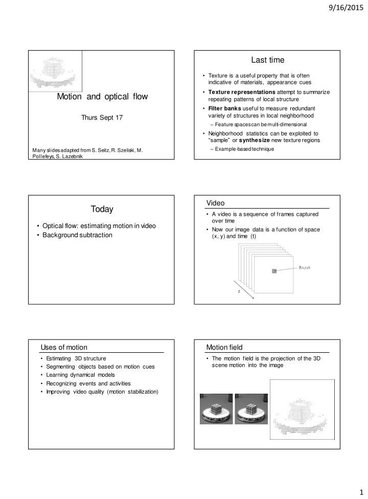
Motion and optical flow

Many slides adapted from S. Seitz, R. Szeliski, M. Pollefeys, S. Lazebnik

Thurs Sept 17

Last time

• Texture is a useful property that is often

indicative of materials, appearance cues

• Texture representations attempt to summarize

repeating patterns of local structure

• Filter banks useful to measure redundant

variety of structures in local neighborhood

– Feature spaces can be multi-dimensional

• Neighborhood statistics can be exploited to

“sample” or synthesize new texture regions

– Example-based technique

Today

• Optical flow: estimating motion in video
• Background subtraction

Video

• A video is a sequence of frames captured
• ver time
• Now our image data is a function of space

(x, y) and time (t)

Uses of motion

• Estimating 3D structure
• Segmenting objects based on motion cues
• Learning dynamical models
• Recognizing events and activities
• Improving video quality (motion stabilization)

Motion field

• The motion field is the projection of the 3D

scene motion into the image

9/16/2015 2

Motion parallax

http://psych.hanover.edu/KRANTZ/MotionParall ax/MotionParallax.html

Figure from Michael Black, Ph.D. Thesis

Length of flow vectors inversely proportional to depth Z of 3d point

points closer to the camera move more quickly across the image plane

Motion field + camera motion

Motion field + camera motion Motion estimation techniques

• Direct methods
• Directly recover image motion at each pixel from spatio-temporal

image brightness variations

• Dense motion fields, but sensitive to appearance variations
• Suitable for video and when image motion is small
• Feature-based methods
• Extract visual features (corners, textured areas) and track them
• ver multiple frames
• Sparse motion fields, but more robust tracking
• Suitable when image motion is large (10s of pixels)

Optical flow

• Definition: optical flow is the apparent motion
• f brightness patterns in the image
• Ideally, optical flow w ould be the same as the

motion field

• Have to be careful: apparent motion can be

caused by lighting changes w ithout any actual motion Apparent motion != motion field

Figure from Horn book

9/16/2015 3

Problem definition: optical flow

How to estimate pixel motion from image H to image I?

• Solve pixel correspondence problem

– given a pixel in H, look for nearby pixels of the same color in I

Key assumptions

• color constancy

: a point in H looks the same in I

– For grayscale images, this is brightness constancy

• small motion: points do not move very far

This is called the optical flow problem

Brightness constancy

Figure by Michael Black

Optical flow constraints

Let’s look at these constraints more closely

• brightness constancy: Q: what’s the equation?
• small motion:

) , ( ) , ( v y u x I y x H   

Optical flow equation

Combining these two equations

Optical flow equation

Q: how many unknowns and equations per pixel?

The aperture problem

Perceived motion

9/16/2015 4

The aperture problem

Actual motion

The barber pole illusion

http://en.wikipedia.org/wiki/Barberpole_illusion

Figure by Michael Black

Solving the aperture problem

• How to get more equations for a pixel?
• Spatial coherence constraint: pretend the pixel’s

neighbors have the same (u,v)

Solving the aperture problem

• How to get more equations for a pixel?
• Spatial coherence constraint: pretend the pixel’s

neighbors have the same (u,v)

• If we use a 5x5 window, that gives us 25 equations per pixel

Slide credit: Steve Seitz

Solving the aperture problem

Prob: we have more equations than unknowns

• The summations are over all pixels in the K x K window
• This technique was first proposed by Lucas & Kanade (1981)

Solution: solve least squares problem

• minimum least squares solution given by solution (in d) of:

Slide credit: Steve Seitz

Conditions for solvability

When is this solvable?

• A

TA should be invertible

• A

TA should not be too small

– eigenvalues l1 and l2 of A

TA should not be too small

• A

TA should be well-conditioned

– l1/ l2 should not be too large (l1 = larger eigenvalue)

Slide by Steve Seitz, UW

9/16/2015 5

Edge

– gradients very large or very small – large l1, small l2

Low-texture region

– gradients have small magnitude

– small l1, small l2

High-texture region

– gradients are different, large magnitudes

– large l1, large l2

(Example applications with optical flow)

Today

• Optical flow: estimating motion in video
• Background subtraction

Video as an “Image Stack”

Can look at video data as a spatio-temporal volume

• If camera is stationary, each line through time corresponds

to a single ray in space

t

255

time

Alyosha Efros, CMU

9/16/2015 6

Input Video

Alyosha Efros, CMU

Average Image

Alyosha Efros, CMU

Birgi T amersoy , UT Austin

Background subtraction

• Simple techniques can do ok with static camera
• …But hard to do perfectly
• Widely used:

– Traffic monitoring (counting vehicles, detecting & tracking vehicles, pedestrians), – Human action recognition (run, walk, jump, squat), – Human-computer interaction – Object tracking

Birgi T amersoy , UT Austin Birgi T amersoy , UT Austin Birgi T amersoy , UT Austin

9/16/2015 7

Birgi T amersoy , UT Austin Birgi T amersoy , UT Austin

Frame differences

• vs. background subtraction
• Toyama et al. 1999

Birgi T amersoy , UT Austin

Average/Median Image

Alyosha Efros, CMU

Background Subtraction

• =

Alyosha Efros, CMU

9/16/2015 8

Pros and cons

Advantages:

• Extremely easy to implement and use!
• All pretty fast.
• Corresponding background models need not be constant,

they change over time. Disadvantages:

• Accuracy of frame differencing depends on object speed

and frame rate

• Median background model: relatively high memory

requirements.

• Setting global threshold Th…

When will this basic approach fail?

Background mixture models

• Adaptive Background Mixture Models for Real-Time Tracking, 1999,
• Chris Stauer & W

.E.L. Grimson

Idea: model each background pixel with a mixture of Gaussians; update its parameters over time.

So far: features and filters

Transforming images; gradients, textures, edges, flow