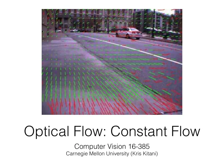
Optical Flow: Constant Flow Computer Vision 16-385 Carnegie Mellon - - PowerPoint PPT Presentation

Optical Flow: Constant Flow

Computer Vision 16-385

Carnegie Mellon University (Kris Kitani)

Given a pair of images Estimate the optical flow field

Optical Flow

(a.k.a., Video Stabilization, Tracking, Stereo Matching, Registration)

{v(pi), u(pi)}

{It, It+1}

spatial derivative

• ptical flow

temporal derivative

Ixu + Iyv + It = 0

Ix = ∂I ∂x Iy = ∂I ∂y u = dx dt v = dy dt It = ∂I ∂t How can we use the brightness constancy equation to estimate the optical flow?

Ixu + Iyv + It = 0

known unknown We need at least ____ equations to solve for 2 unknowns.

Ixu + Iyv + It = 0

known unknown Where do we get more equations (constraints)?

Ixu + Iyv + It = 0

Where do we get more equations (constraints)? Assume that the surrounding patch (say 5x5) has ‘constant flow’

Flow is locally smooth Neighboring pixels have same displacement

Using a 5 x 5 image patch, gives us 25 equations Assumptions:

Flow is locally smooth Neighboring pixels have same displacement

Using a 5 x 5 image patch, gives us 25 equations Assumptions:

Ix(p1)u + Iy(p1)v = −It(p1) Ix(p2)u + Iy(p2)v = −It(p2) . . . Ix(p25)u + Iy(p25)v = −It(p25)

Flow is locally smooth Neighboring pixels have same displacement

Using a 5 x 5 image patch, gives us 25 equations 2 6 6 6 4 Ix(p1) Iy(p1) Ix(p2) Iy(p2) . . . . . . Ix(p25) Iy(p25) 3 7 7 7 5  u v

• = −

2 6 6 6 4 It(p1) It(p2) . . . It(p25) 3 7 7 7 5 Assumptions: Matrix form

Flow is locally smooth Neighboring pixels have same displacement

Using a 5 x 5 image patch, gives us 25 equations 2 6 6 6 4 Ix(p1) Iy(p1) Ix(p2) Iy(p2) . . . . . . Ix(p25) Iy(p25) 3 7 7 7 5  u v

• = −

2 6 6 6 4 It(p1) It(p2) . . . It(p25) 3 7 7 7 5

A

x

b

25 × 2

2 × 1

25 × 1

How many equations? How many unknowns? How do we solve this?

Assumptions:

Least squares approximation

ˆ x = arg min

x

||Ax − b||2 A>Aˆ x = A>b

is equivalent to solving

To obtain the least squares solution solve:

Least squares approximation

ˆ x = arg min

x

||Ax − b||2 A>Aˆ x = A>b

is equivalent to solving

2 4 P

p∈P

IxIx P

p∈P

IxIy P

p∈P

IyIx P

p∈P

IyIy 3 5  u v

• = −

2 4 P

p∈P

IxIt P

p∈P

IyIt 3 5 where the summation is over each pixel p in patch P

A>A A>b

ˆ x

x = (A>A)1A>b

To obtain the least squares solution solve:

Least squares approximation

ˆ x = arg min

x

||Ax − b||2 A>Aˆ x = A>b

is equivalent to solving

2 4 P

p∈P

IxIx P

p∈P

IxIy P

p∈P

IyIx P

p∈P

IyIy 3 5  u v

• = −

2 4 P

p∈P

IxIt P

p∈P

IyIt 3 5 where the summation is over each pixel p in patch P

A>A A>b

ˆ x

Sometimes called ‘Lucas-Kanade Optical Flow’
 (can be interpreted to be a special case of the LK method with a translational warp model)

A>Aˆ x = A>b

When is this solvable? ATA should be invertible ATA should not be too small ATA should be well conditioned

λ1 and λ2 should not be too small λ1/λ2 should not be too large (λ1=larger eigenvalue)

2 4 P

p∈P

IxIx P

p∈P

IxIy P

p∈P

IyIx P

p∈P

IyIy 3 5 Where have you seen this before?

A>A =

2 4 P

p∈P

IxIx P

p∈P

IxIy P

p∈P

IyIx P

p∈P

IyIy 3 5 Where have you seen this before? Harris Corner Detector!

Implications

• Corners are when λ1, λ2 are big; this is also when

Lucas-Kanade optical flow works best

• Corners are regions with two different directions of

gradient (at least)

• Corners are good places to compute flow!

What happens when you have no ‘corners’?

You want to compute optical flow. What happens if the image patch contains only a line?

ApertureProblem

In which direction is the line moving?

small visible image patch

ApertureProblem

In which direction is the line moving?

small visible image patch

ApertureProblem

ApertureProblem

ApertureProblem

ApertureProblem

Want patches with different gradients to the avoid aperture problem

Want patches with different gradients to the avoid aperture problem

1 1 1 1 2 2 2 2 3 3 3 3 4 4 4 4 5 5 5 5

• 1

1 1

• 2

2 2

• 3

3 3

• 4

4 4

y x y x

• ptical flow: (1,1)

H(x,y) = y I(x,y)

It(3, 3) = I(3, 3) − H(3, 3) = −1

Ixu + Iyv + It = 0

Iy(3, 3) = 1

Ix(3, 3) = 0

v = 1

We recover the v of the optical flow but not the u. This is the aperture problem.

Compute gradients Solution: