More Raster Line Issues Fat lines with multiple pixel width - PDF document

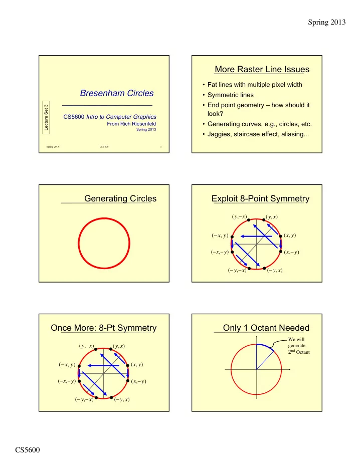
Spring 2013 More Raster Line Issues • Fat lines with multiple pixel width Bresenham Circles • Symmetric lines • End point geometry – how should it Lecture Set 3 look? CS5600 Intro to Computer Graphics • Generating curves, e.g., circles, etc. From Rich Riesenfeld Spring 2013 • Jaggies, staircase effect, aliasing... Spring 2013 CS 5600 1 Generating Circles Exploit 8-Point Symmetry y  ( , x ) ( y , x )  ( , ) ( , ) x y x y  x  x  ( , y ) ( , ) y  y   ( , ) x ( y , x ) Once More: 8-Pt Symmetry Only 1 Octant Needed We will y  ( , x ) ( , ) generate y x 2 nd Octant  ( , ) ( , ) x y x y  x  x  ( , y ) ( , ) y  y   ( , x ) ( y , x ) CS5600

Spring 2013 2 nd Octant Is a Good Arc Generating pt ( x , y ) gives the following 8 pts by symmetry: • It is a function in this domain – single-valued {( x , y ) , (- x , y ) , (- x ,- y ) , ( x ,- y ), – no vertical tangents: | slope |  1 ( y , x ) , (- y , x ) , (- y ,- x ) , ( y ,- x )} • Lends itself to Bresenham – only need consider E or SE Implicit Eq’s for Circle Choose E or SE • Let F ( x,y ) = x 2 + y 2 – r 2 • Function is x 2 + y 2 – r 2 = 0 • For ( x,y ) on the circle, F ( x,y ) = 0 • So, F ( M )  0  SE • So, F ( x,y ) > 0  ( x,y ) Outside • And, F ( M ) < 0  E • And, F ( x,y ) < 0  ( x,y ) Inside F ( M ) < 0  E F ( M )  0  SE E E ideal curve ideal   M M curve SE SE CS5600

Spring 2013 Look at Case 1: E Decision Variable d E ideal Again, we let, curve  d = F ( M ) M SE d old < 0  E d old < 0  E    1    1 ( 1, ) d F y F ( 2, ) x d y x p old p p 2 new p 2 2 2 2 2    1 2  1     ( 1)   2 ( 2) ( ) ( ) y x y x r p p r p p 2 2 d old < 0  E d old < 0  E    (2 3) d d    x , new old p d d E new old  Since, d d where, new old   2 2           2 3 ( 2 ) ( 1 ) 2 2 x x p x p ( 4 4 ) ( 2 1 ) x p x p x p x p E p   2 3 x p CS5600

Spring 2013 d old  0  SE Look at Case 2: SE    3 ( 2, ) F y d x p new p 2 E 2 2     3  2 ( 2) ( ) x y r p ideal p 2  M curve     (2 2 5) y d d x new old p p Because,…, straightforward manipulation SE d old  0  SE d old  0  SE  d   d  d d new old new old     3 1 3 1                   2 2 2 2 2 2 2 2 2 2 2 2 ( 2 ) ( y p ) r ( 1 ) ( y p ) r ( 2 ) ( y p ) r ( 1 ) ( y p ) r x p  x p  x p  x p  x x     2 2 2 2     9 1 9 1               2 2 2 2 ( 3 ) 3   ( 3 ) 3   = 2 y p y p y p y p = 2 y p y p y p y p x p x p 4 4 4 4     d old  0  SE d old  0  SE  d   d  d d new old new old 1   9 3 1                 2 2 2 2 2 2 ( 2 3 ) ( 3 ) ( ( 2 ) ( ) r ( 1 ) ( ) r y p y p ) y p  y p  x p x p x x p x   2 2 4 4                  9 1        2 2  E ( 3 ) 3   = 2 y p y p y p y p x p x From From new From old x 4 4   calculation y-coordinate y-coordinate CS5600

Spring 2013 d old  0  SE Note: ∆΄ s Not Constant I.e.,     (2 2 5) y d d x   new old p p and E SE    d old SE depend on values of x p and y p     2 2 5 y x SE p p Summary Initial Condition • ∆΄ s are no longer constant over entire line • Let r be an integer. Start at ( 0 , r ) 1  • Algorithm structure is exactly the same • Next midpoint M lies at ( 1 , r ) 2 • Major difference from the line algorithm 1 1 • So,    2    2 F ( 1 , r ) 1 ( r ) r r – ∆ is re-evaluated at each step 2 4 – Requires real arithmetic 5   r 4 Ellipses Getting to Integers • Note the previous algorithm • Evaluation is analogous involves real arithmetic • Structure is same • Can we modify the algorithm to use • Have to work out the ∆΄ s integer arithmetic? CS5600

Spring 2013 Integer Circle Algorithm Integer Circle Algorithm • Define a shift decision variable • Now, the initialization is h = 1 - r 1  d  h • So the initial value becomes 4 1 1 ) 1 5 1  h       • In the code, plug in ( 1 , F r ( r ) d 2 4 4 4 4   1 r Integer Circle Algorithm Integer Circle Algorithm 1    • But, h begins as an integer • Then, 0 becomes h d 4 • And, h gets incremented by integer • Since h an integer • Hence, we have an integer circle algorithm 1     h 0 h • Note: Sufficient to test for h < 0 4 End of Bresenham Circles Another Digital Line Issue • Clipping Bresenham lines • The integer slope is not the true slope • Have to be careful • More issues to follow CS5600

Spring 2013 Clipped Line Line Clipping Problem x  y  x  y x x max max min ( x , y ) 1 1 ( x , ) y 1 1 Clipping Rectangle   ( x , y ) Clipping 0 0 Rectangle y  ( y x , ) y min 0 0 y  y x  x  x x min max min Clipped Line Has Different Slope ! Drawing Clipped Lines ( x , y ) 1 1 m  1 2 ( x , ) y 0 0 m  34 Pick Right Slope to Reproduce Pick Right Slope to Reproduce Original Line Segment Original Line Segment Zoom of previous situation Zoom of previous situation CS5600

Spring 2013 Clipping Against y = y min Clipping Against x = x min x  x min x  x NE Line getting min clipped  ( )) A x , Round ( m x B B min min            y  midpoint M y min E 1  y min  y Clip Rectangle Clip Rectangle y           2 y min  ( )) x , ( m x B  y min min min  y 1 Clipping Against y = y min Clipping Against y = y min • Use Line ∩ y = y min - ½ • Situation is complicated • Multiple pixels involved at ( y = y min ) • Round up to nearest integer x • Want all of those pixels as “ in ” • Analytic ∩ , rounding x gives A • This yields point B , the desired result • We want point B Jaggies and Aliasing Jaggies-Manifestation of Aliasing • To represent a line with discrete pixel values is to sample finitely a continuous function • Jaggies are visual manifestation, artifacts, resulting from information loss • The term aliasing is a complicated, unintuitive phenomenon which will be Added resolution helps, but does not directly defined later address underlying issue of aliasing CS5600

Spring 2013 Jaggies and Aliasing Anti-aliasing • Doubling resolution in x and y Pixel 5 reduces the effect of the problem, Space 4 3 but does not fix it 2 • Doubling resolution costs 4 times 1 0 memory, memory bandwidth and 0 1 2 3 4 5 6 7 8 9 10 11 scan conversion time! Pixel intensity (darkness, in this case) is proportional to area covered by line Anti-aliasing Anti-aliasing • Set each pixel’s intensity value Pixel Space proportional to its area of overlap (i.e. sub-area) covered by primitive • Not more than 1 pixel/column for lines with 0 < slope < 1 Pixel intensity (darkness, in this case) is proportional to area covered by line Gupta-Sproull Algorithm -1 Gupta-Sproull Algorithm -2 • Use coarse (4-bit, say) lookup table for • Standard Bresenham chooses E or NE intensity : Filter ( D, t ) • Incrementally compute distance D from • Note, Filter value depends only on D chosen pixel to center of line and t , not the slope of line ! (Very clever) • Vary pixel intensity by value of D • For line _ width t = 1 geometry and • Do this for line above and below associated calculations greatly simplify CS5600

Spring 2013 Cone Filter for Weighted Observations Area Sampling    • Lines are complicated r  1 • Many aspects to consider    D • We omitted many    • What about intensity of       vs y = 0 ? y = x t  1 Unit thickness line intersects no more than 3 pixels The End Bresenham Circles Lecture Set 3 CS5600