Mining molecular flexibility: novel tools, novel insights F. Cazals, - - PowerPoint PPT Presentation

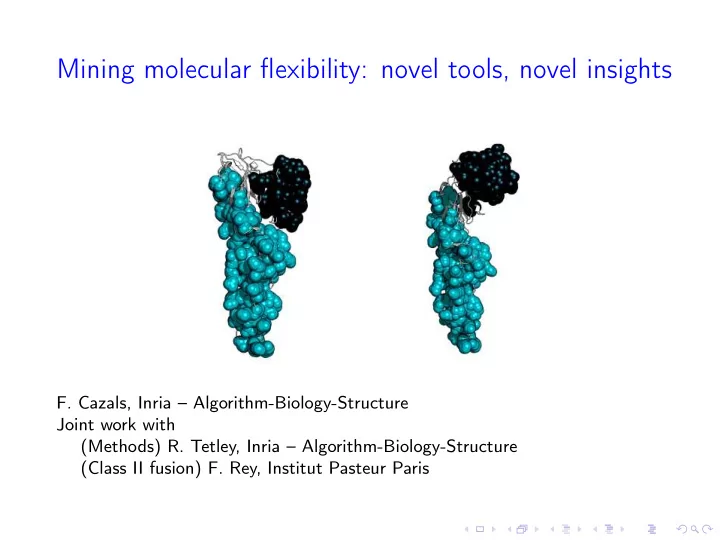
Mining molecular flexibility: novel tools, novel insights

• F. Cazals, Inria – Algorithm-Biology-Structure

Joint work with (Methods) R. Tetley, Inria – Algorithm-Biology-Structure (Class II fusion) F. Rey, Institut Pasteur Paris

Mining molecular flexibility: novel tools, novel insights

Introduction Multiscale analysis of structurally conserved motifs Combined RMSD The Structural Bioinformatics Library Outlook Multiscale analysis of structurally conserved motifs Technicalities

Challenge Dynamics of proteins: specification

⊲ Input: structure(s) of biomolecules + potential energy model ⊲ Output ◮ Thermodynamics: meta-stable states and observables ◮ Dynamics: Markov state model – requires rare transition events ⊲ Time-scales ◮ Biological time-scale > millisecond ◮ Integration time step in molecular dynamics: ∆t ∼ 10−15s ◮ 5.058ms of

simulation time; ◮ ∼ 230 GPU years on NVIDIA GeForce GTX 980 proc.

⊲Ref:

Chodera et al, eLife, 2019

Mining molecular flexibility: novel tools, novel insights

Introduction Multiscale analysis of structurally conserved motifs Combined RMSD The Structural Bioinformatics Library Outlook Multiscale analysis of structurally conserved motifs Technicalities

Combined RMSD : TBEV glycoprotein in two different conformations pre and post fusion

⊲ Classical analysis: Statistics from Apurva: ◮ 370 a.a. aligned ◮ lRMSD: 11.1Å ⊲ Our motifs: Motif Alignment size lRMSD Large 88 1.69 Small 40 0.38

Structural Motif

⊲ Input: We are given two polypeptide chains SA and SB

Definition 1.

Given two sets of a.a. MA = {ai1, . . . , ais } ⊂ SA and MB = {bi1, . . . , bis } ⊂ SB, and a one-to-one alignment {(aij ↔ bij )} between them, we define the least RMSD ratio as follows: rlRMSD(MA, MB) = lRMSD(MA, MB)/lRMSD(SA, SB). (1) The sets MA and MB are called structural motifs provided that |MA| = |MB| ≥ s0 and rlRMSD(MA, MB) ≤ r0, for appropriate thresholds s0 and r0.

Key idea: exploiting quasi-isometric deformations to identify almost rigid | isometric regions in structures

⊲ Quasi-isometric deformation: (selected) distances (almost) preserved

d1 d2 d3 d′

1

d′

3

d′

2

d1 ∼ d′

1

d2 ∼ d′

2

d3 = d′

3 ⊲ Tracking such deformation may be done at two scales: ◮ Global preservation: maximal cliques – NP-hard problem. ◮ Local preservation: spanning trees connecting atoms whose relative distances are conserved.

Multi-scale rigidity: embodied in the notion of filtration

⊲ Key ideas ◮ Filtration: sequence of nested topological space – read: sequence of nested sets of amino-acids ◮ Ordering of a.a.: by decreasing rigidity index – those involved in rigid blocks come first

Motifs for two structures A and B: a generic approach

◮ Step 1: use an aligner for the seed alignment and scores

◮ (A and B) Compute a seed alignment ◮ (A, then B) Sort residues by decreasing structural conservation

◮ Step 2: use a filtration to perform a multiscale analysis

◮ (A, then B) Identify structurally conserved regions

◮ Step 3: reuse the aligner to bootstrap the alignment

◮ (A and B) Re-compute a structural alignment between pairs of regions

Build filtrations:

• from conserved distances (CD)
• from space filling diagram (SFD)

For each chain: build the per- sistence diagram of connected components of the filtration Identification of struc- tural motifs

Step 2: Filtrations and persistence diagrams Step 3: Identifying structural motifs

Death Birth

Given two structures, compute a pairwise structural alignment

Step 1: Seed alignments, scores

Statistical assessment

• f structural motifs

Step 4: Filtering structural motifs

sij = |dA

ij − dB ij|

Compute distance conservation scores Hierarchical representation with Hasse diagrams

⊲ NB: s is the distance variation | D (t, t′) | applied to C carbons.

Generic method: instantiations

⊲ Main steps: ◮ step 1 ≡ alignment to rigidity scores; ◮ step 2 ≡ rigidity scores to filtrations; ◮ step 3 ≡ filtrations to motifs via local alignments. ⊲ Ingredient 1: an aligner for steps 1 and 3 ◮ Options: Kpax, Apurva, (FATCAT) ⊲ Ingredient 2: filtration encoding based on rigidity scores ◮ Option 1: based on conserved distances (cf Kruskal’s MST algorithm) ◮ Option 2: based on space filling diagrams (Voronoi / α-shapes) ⊲ Resulting programs: Align-Kpax-CD, Align-Kpax-SFD, Align-Apurva-CD, Align-Apurva-SFD ⊲ Nb: conformation vs homologous proteins: (trivial) alignment

Motifs reveal the multi-scale structural conservation within global alignments

⊲ Size of motifs vs lRMSD on challenging cases 1BGE vs 2GMF 1CEW vs 1MOL 1CID vs 2RHE 1CRL vs 1EDE ⊲Ref:

Pairs of structures: from Godzik et al, Bioinformatics, 2003

Mining molecular flexibility: novel tools, novel insights

Introduction Multiscale analysis of structurally conserved motifs Combined RMSD The Structural Bioinformatics Library Outlook Multiscale analysis of structurally conserved motifs Technicalities

Comparing two molecules: the combined RMSD

⊲ Rationale: use one rigid motion for each rigid/structurally conserved region ⊲ Motifs for two molecules A and B, and their intersection graph

A1 A2 A3 A4 A5 A6 B1 B2 B3 B4 B5 M (A)

1

M (A)

2

M (A)

3

M (B)

1

M (B)

2

M (B)

3

Definition 2.

Consider two structures A and B for which non-overlapping domains {C (A)

i

, C (B)

i

}i=1,...,m have been identified. Assume that a lRMSD has been computed for each pair (C (A)

i

, C (B)

i

). Let wi be the weights associated with an individual lRMSD . The combined RMSD is defined by RMSDComb.(A, B) =

• m
• i=1

wi

• i wi

lRMSD2(C (A)

i

, C (B)

i

). (2) ⊲ Rmk: comes into two guises, namely vertex weighted and edge weighted

Combined RMSD : TBEV glycoprotein in two different conformations pre and post fusion

⊲ Classical analysis: Statistics from Apurva: ◮ 370 a.a. aligned ◮ lRMSD: 11.1Å ⊲ Our motifs: Motif Alignment size lRMSD Large 88 1.69 Small 40 0.38

Mining molecular flexibility: novel tools, novel insights

Introduction Multiscale analysis of structurally conserved motifs Combined RMSD The Structural Bioinformatics Library Outlook Multiscale analysis of structurally conserved motifs Technicalities

The Structural Bioinformatics Library

http://sbl.inria.fr ⊲Ref:

Cazals and Dreyfus; Bioinformatics, 2016

SBL and Jupyter notebooks: guided tour

http://sbl.inria.fr/applications

Mining molecular flexibility: novel tools, novel insights

Introduction Multiscale analysis of structurally conserved motifs Combined RMSD The Structural Bioinformatics Library Outlook Multiscale analysis of structurally conserved motifs Technicalities

Summary and outlook

⊲ Combined RMSD – RMSDComb. ◮ Structural comparisons based on (relatively) independent sets ⊲ Multiscale analysis of structural conservation ◮ Segregating dof (internal coords.) into active and passive ◮ Towards more efficient algorithms for thermodynamics - dynamics ⊲ Software: all tools in the SBL ⊲ Ongoing ◮ Design of move sets ◮ Applications to energy landscapes: exploration, thermodynamics

Bibliography

• Combined RMSD: [1]
• Structural motifs: [2]
• Software: [3]
• Partition functions [4]
• Cluster matching: [5]
• F. Cazals and R. Tetley.

Characterizing molecular flexibility by combining lRMSD measures. Proteins, 87(5):380–389, 2019.

• F. Cazals and R. Tetley.

Multiscale analysis of structurally conserved motifs. 2019. Submitted.

• F. Cazals and T. Dreyfus.

The Structural Bioinformatics Library: modeling in biomolecular science and beyond. Bioinformatics, 7(33):1–8, 2017.

• A. Chevallier and F. Cazals.

Wang-landau algorithm: an adapted random walk to boost convergence.

• J. of Computational Physics (Under revision), 2019.
• F. Cazals, D. Mazauric, R. Tetley, and R. Watrigant.

Comparing two clusterings using matchings between clusters of clusters. ACM J. of Experimental Algorithms, 24(1):1–42, 2019.

Mining molecular flexibility: novel tools, novel insights

Introduction Multiscale analysis of structurally conserved motifs Combined RMSD The Structural Bioinformatics Library Outlook Multiscale analysis of structurally conserved motifs Technicalities

Mining molecular flexibility: novel tools, novel insights

Introduction Multiscale analysis of structurally conserved motifs Combined RMSD The Structural Bioinformatics Library Outlook Multiscale analysis of structurally conserved motifs Technicalities

Step 1: rigidity score as Cα ranks for chains A and B

⊲ Input: a structural alignment yields ◮ dA

i,j: dist. between Cα i and j on

chain A ◮ dB

i,j: dist. between Cα i and j on

chain B

i j Chain A Chain B dA

i,j

dB

i,j

⊲ Distance difference matrix between A and B: sij =| dA

i,j − dB i,j |, i = 1, . . . , N, j = 1, . . . , N.

(3) ⊲ Cα rank of residue i: index of the smallest sij involving this residue in the sorted sequence Sorted{sij}. Assuming the ordering of scores depicted, the ranks are as follows: ◮ one for C1 and C2 ◮ two for C3 and C4 ◮ likewise for the second chain.

a1 a2 a3 a4 b1 b2 b4 b3 Sorted scores: s12 < s34 < s23 < s13 < s14 < s24

Step 1: illustration for 1SVB - 1URZ

⊲ Plots: ◮ Cα distance plot: for chain A, the function dA

i,j (or dB i,j) as a function of

the Cα rank. ◮ Sequence shift plot: for chain A (or chain B), the function j − i as a function of the Cα rank. ◮ Score plot: score sij as a function of the Cα rank.

Step 2a – filtration using Space Filling Diagrams

building the filtration

⊲ Filtration = sequence of nested sets ⊲ Model a collection of amino-acids with its Solvent Accessible Surface ⊲ For both structures, independently: ◮ insert a.a. by increasing Cα ranks, ◮ maintain the corresponding space filling model of the Solvent Accessible Model

(A) A(1) A(2) A(3) A(4) A(5) A(6)

Step 2a – filtration using Space Filling Diagrams

persistence diagram of the connected components

⊲ Assessing the stability of conserved regions: ◮ compute its connected components ◮ maintain the associated persistence diagram

(A) (B) A(1) A(2) A(3) A(4) A(5) A(6) A(1) A(2) A(3) A(4) A(5) A(6) A(7)

2 6 7 8

(D) (C)

Birth Death

c.c. involving A(6) c.c. involving A(2), A(3), A(4), A(5), A

y = x

A(1) A(2) A(3) A(4) A(5) A(6) A(7) A(8)

Step 3: identifying motifs – rationale

⊲ Motifs from local structural alignments inferred from the PD: ◮ points nearby in the pers. diag. have a comparable rigidity signature ◮ each such point corresponds to a set of a.a. in one structure ◮ therefore: run a local alignment between these regions

◮ motif: rlRMSD ≤ r0 and |MA| = |MB| ≥ s0

⊲ Topological changes and accretion: ◮ accretion: insertion of an a.a. connected to an already existing connected component. ◮ concomitant birth and death i.e. 0-persistence i.e. point on the diagonal of the PD for c.c. ◮ pitfall: accretion may be such that a PD has very few points!

Step 3: identifying motifs – details

⊲ Identifying motifs: – For each critical value (death date) t of either persistence diagram: – compute the c.c. FA = {c1, . . . , cnA} of F A

t

– compute the c.c. FB = {c′

1, . . . , c′ nB } of F B t

– (simple) compute a structural alignment for each pair (ci, c′

j ) ∈ FA × FB

– (involved) solve a k-partition matching for FA and FB, and run a structural alignment on the resulting meta-clusters ⊲ Filtering motifs: ◮ compute the Hasse diagram (for the inclusion) of the motifs found NB: inclusion owes to the nested-ness of sublevel ets. ◮ retain the roots of the Hasse diagrams only.

Steps 2-3: illustration for 1SVB - 1URZ

⊲ Step 2, Building the filtration and its persistence diagram (Align-Identity-CD) ⊲ Step 3, Computing structural motifs with bootstrap: run a local alignment for regions associated with connected components defined by critical values in the persistence diagram