SLIDE 7 7
FASTA in a picture
- Proc. Natl. Acad. Sci. USA 85 (1988)
2445 A
50 100
50 100 50
100
N
''
\X\\\'
*
\\'
\\ \\ *
'~\'
\
C50
100
B
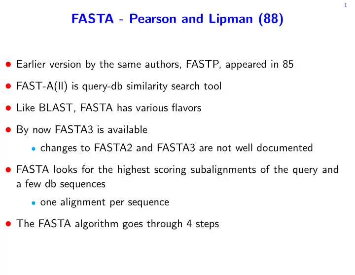
Identification of sequence similarities by FASTA. The
four steps used by the FASTA program to calculate the initial and
- ptimal similarity scores between two sequences are shown. (A)
Identify regions of identity. (B) Scan the regions using a scoring
matrix and save the best initial regions. Initial regions with scores
less than the joining threshold (27) are dashed. The asterisk denotes
the highest scoring region reported by FASTP. (C) Optimally join
initial regions with scores greater than a threshold. The solid lines
denote regions that are joined to make up the optimized initial score. (D) Recalculate an optimized alignment centered around the highest scoring initial region. The dotted lines denote the bounds of the
- ptimized alignment. The result of this alignment is reported as the
- ptimized score.
much closer to the optimized score for many sequences. In
fact, unlike FASTP, the FASTA method may yield initial
scores that are higher than the corresponding optimized
scores.
Local Similarity Analyses. Molecular biologists are often interested in the detection of similar subsequences within longer sequences. In contrast to FASTP and FASTA, which
report only the one highest scoring alignment between two
sequences, local sequence comparison tools can identify
multiple alignments between smaller portions of two
se-
- quences. Local similarity searches can clearly show the
results of gene duplications (see Fig. 2) or repeated struc- tural features (see Fig. 3) and are frequently displayed using
a "graphic matrix" plot (7), which allows one to detect
regions of local similarity by eye. Optimal algorithms for
sensitive local
sequence comparison (6, 8, 9) can have
tremendous computational requirements in time and mem-
- ry, which make them impractical on microcomputers and,
when comparing longer sequences, on larger machines as
well.
The program for detecting local similarities, LFASTA,
uses the same first two steps for finding initial regions that
FASTA uses. However, instead of saving 10 initial regions, LFASTA saves all diagonal regions with similarity scores
greater than a threshold. LFASTA and FASTA also differ in
the construction of optimized alignments. Instead of focus- ing on a single region, LFASTA computes a local alignment
for each initial region. Thus LFASTA considers all of the
initial regions shown in Fig. 1B, instead of just the diagonal
shown in Fig. 1D. Furthermore, LFASTA considers not
50 100
- nly the band around each initial region but also potential
sequence alignments for some distance before and after the
initial region. Starting at the end of the initial region, an
- ptimization (6) proceeds in the reverse direction until all
possible alignment scores have gone to zero. The location of the maximal local similarity score in the reverse direction is then used to start a second optimization that proceeds in the
forward direction. An optimal path starting from the forward
maximum is then displayed (5). The local homologies can be
displayed as sequence alignments (see Fig. 2B) or on a two-dimensional graphic matrix style plot (see Figs. 2A and
3).
Statistical Significance. The rapid sequence comparison
algorithms we have developed also provide additional tools
for evaluating the statistical significance of an alignment.
There are approximately 5000 protein sequences, with 1.1
million amino acid residues, in the NBRF protein sequence
library, and any computer program that searches the library
by calculating a similarity score for each sequence in the
library will find a highest scoring sequence, regardless of
whether the alignment between the query and library se-
quence is biologically meaningful or not. Accompanying the
previous version of FASTP was a program for the evaluation
- f statistical significance, RDF, which compares one se-
quence with randomly permuted versions of the potentially
related sequence.
We have written a new version of RDF (RDF2) that has
several improvements. (i) RDF2 calculates three scores for
each shuffled sequence: one from the best single initial region
(as found by FASTP), a second from the joined initial regions
(used by FASTA), and a third from the optimized diagonal.
(it) RDF2 can be used to evaluate amino acid or DNA
sequences and allows the user to specify the scoring matrix to
be employed. Thus
sequences found using the PAM250
scoring matrix can be evaluated using the identity or genetic
code matrix. (iii) The user may specify either a global or local
shuffle routine.
Locally biased amino acid or nucleotide composition is perhaps the most common reason for high similarity scores
- f dubious biological significance (10). High scoring align-
ments between query and library sequences may be due to
patches of hydrophobic or charged amino acid residues or to
A + T- or G + C-rich regions in DNA. A simple Monte Carlo
shuffle analysis that constructs random sequences by taking
each residue in one sequence and placing it randomly along
the length of the new sequence will break up these patches of biased composition. As a result, the scores of the shuffled
sequences may be much lower than those of the unshuffled sequence, and the sequences will appear to be related.
Alternatively, shuffled sequences can be constructed by
permuting small blocks of 10 or 20 residues so that, while the
- rder of the sequence is destroyed, the local composition is
- not. By shuffling the residues within short blocks along the
sequence, patches of G + C- or A + T-rich regions in DNA,
for example, are undisturbed. Evaluating significance with a local shuffle is more stringent than the global approach, and there may be some circumstances in which both should be
used in conjunction. Whereas two proteins that share a
common evolutionary ancestor may have clearly significant
similarity scores using either shuffling strategy, proteins related because of secondary structure or hydropathic pro-
file may have similarity scores whose significance decreases
dramatically when the results of global and local shuffling
are compared.
- Implementation. The FASTA/LFASTA package of se-
quence analysis tools is written in the C programming lan- guage and has been implemented under the Unix, VAX/
VMS, and IBM PC DOS operating systems. Versions of the
program that run on the IBM PC are limited to query se-
50 100.
\l
6F
1 I I
Biochemistry: Pearson and Lipman
16