frequent pattern mining
play

Frequent Pattern Mining Frequent Sequence Mining Frequent Tree - PowerPoint PPT Presentation

Overview Frequent Pattern Mining comprises Frequent Item Set Mining and Association Rule Induction Frequent Pattern Mining Frequent Sequence Mining Frequent Tree Mining Christian Borgelt Frequent Graph Mining Dept. of Mathematics


  1. Reminder: Partially Ordered Sets Properties of the Support of Item Sets • A partial order is a binary relation ≤ over a set S which satisfies ∀ a, b, c ∈ S : Monotonicity in Calculus and Mathematical Analysis ◦ a ≤ a (reflexivity) • A function f : I R → I R is called monotonically non-decreasing if ∀ x, y : x ≤ y ⇒ f ( x ) ≤ f ( y ). ◦ a ≤ b ∧ b ≤ a ⇒ a = b (anti-symmetry) • A function f : I R → I R is called monotonically non-increasing ◦ a ≤ b ∧ b ≤ c ⇒ a ≤ c (transitivity) if ∀ x, y : x ≤ y ⇒ f ( x ) ≥ f ( y ). • A set with a partial order is called a partially ordered set (or poset for short). Monotonicity in Order Theory • Let a and b be two distinct elements of a partially ordered set ( S, ≤ ). • Order theory is concerned with arbitrary (partially) ordered sets. ◦ if a ≤ b or b ≤ a , then a and b are called comparable . The terms increasing and decreasing are avoided, because they lose their pictorial motivation as soon as sets are considered that are not totally ordered. ◦ if neither a ≤ b nor b ≤ a , then a and b are called incomparable . • A function f : S → R , where S and R are two partially ordered sets, is called • If all pairs of elements of the underlying set S are comparable, monotone or order-preserving if ∀ x, y ∈ S : x ≤ S y ⇒ f ( x ) ≤ R f ( y ). the order ≤ is called a total order or a linear order . • A function f : S → R is called • In a total order the reflexivity axiom is replaced by the stronger axiom: anti-monotone or order-reversing if ∀ x, y ∈ S : x ≤ S y ⇒ f ( x ) ≥ R f ( y ). ◦ a ≤ b ∨ b ≤ a (totality) • In this sense the support of item sets is anti-monotone . Christian Borgelt Frequent Pattern Mining 13 Christian Borgelt Frequent Pattern Mining 14 Properties of Frequent Item Sets Reminder: Partially Ordered Sets and Hasse Diagrams • A subset R of a partially ordered set ( S, ≤ ) is called downward closed • A finite partially ordered set ( S, ≤ ) can be depicted as a (directed) acyclic graph G , if for any element of the set all smaller elements are also in it: which is called Hasse diagram . ∀ x ∈ R : ∀ y ∈ S : y ≤ x ⇒ y ∈ R • G has the elements of S as vertices. The edges are selected according to: In this case the subset R is also called a lower set . a b c d e If x and y are elements of S with x < y • The notions of upward closed and upper set are defined analogously. (that is, x ≤ y and not x = y ) and ab ac ad ae bc bd be cd ce de there is no element between x and y • For every s min the set of frequent item sets F T ( s min ) is downward closed w.r.t. the partially ordered set (2 B , ⊆ ), where 2 B denotes the powerset of B : (that is, no z ∈ S with x < z < y ), abc abd abe acd ace ade bcd bce bde cde then there is an edge from x to y . ∀ s min : ∀ X ∈ F T ( s min ): ∀ Y ⊆ B : Y ⊆ X ⇒ Y ∈ F T ( s min ). • Since the graph is acyclic abcd abce abde acde bcde • Since the set of frequent item sets is induced by the support function, (there is no directed cycle), the notions of up- or downward closed are transferred to the support function: the graph can always be depicted abcde such that all edges lead downward. Any set of item sets induced by a support threshold s min is up- or downward closed. Hasse diagram of (2 { a,b,c,d,e } , ⊆ ). F T ( s min ) = { S ⊆ B | s T ( S ) ≥ s min } ( frequent item sets) is downward closed, • The Hasse diagram of a total order (Edge directions are omitted; G T ( s min ) = { S ⊆ B | s T ( S ) < s min } (infrequent item sets) is upward closed. (or linear order) is a chain. all edges lead downward.) Christian Borgelt Frequent Pattern Mining 15 Christian Borgelt Frequent Pattern Mining 16

  2. Searching for Frequent Item Sets Searching for Frequent Item Sets • The standard search procedure is an enumeration approach , Hasse diagram for five items { a, b, c, d, e } = B : Idea: Use the properties that enumerates candidate item sets and checks their support. of the support to organize the search for all frequent • It improves over the brute force approach by exploiting the apriori property item sets, especially the to skip item sets that cannot be frequent because they have an infrequent subset. apriori property : a b c d e • The search space is the partially ordered set (2 B , ⊆ ). ∀ I : ∀ J ⊃ I : s T ( I ) < s min • The structure of the partially ordered set (2 B , ⊆ ) helps to identify ab ac ad ae bc bd be cd ce de ⇒ s T ( J ) < s min . those item sets that can be skipped due to the apriori property. ⇒ top-down search (from empty set/one-element sets to larger sets) Since these properties re- abc abd abe acd ace ade bcd bce bde cde late the support of an item • Since a partially ordered set can conveniently be depicted by a Hasse diagram , set to the support of its we will use such diagrams to illustrate the search. subsets and supersets , abcd abce abde acde bcde it is reasonable to organize • Note that the search may have to visit an exponential number of item sets. the search based on the In practice, however, the search times are often bearable, structure of the partially (2 B , ⊆ ) abcde ordered set (2 B , ⊆ ). at least if the minimum support is not chosen too low. Christian Borgelt Frequent Pattern Mining 17 Christian Borgelt Frequent Pattern Mining 18 Hasse Diagrams and Frequent Item Sets Hasse diagram with frequent item sets ( s min = 3): transaction database 1: { a, d, e } 2: { b, c, d } 3: { a, c, e } a b c d e 4: { a, c, d, e } 5: { a, e } The Apriori Algorithm 6: { a, c, d } ab ac ad ae bc bd be cd ce de 7: { b, c } [Agrawal and Srikant 1994] 8: { a, c, d, e } 9: { b, c, e } abc abd abe acd ace ade bcd bce bde cde 10: { a, d, e } abcd abce abde acde bcde Blue boxes are frequent item sets, white boxes infrequent item sets. abcde Christian Borgelt Frequent Pattern Mining 19 Christian Borgelt Frequent Pattern Mining 20

  3. Searching for Frequent Item Sets The Apriori Algorithm 1 Possible scheme for the search: function apriori ( B, T, s min ) begin ( ∗ — Apriori algorithm ∗ ) • Determine the support of the one-element item sets (a.k.a. singletons) k := 1; ( ∗ initialize the item set size ∗ ) and discard the infrequent items / item sets. � E k := i ∈ B {{ i }} ; ( ∗ start with single element sets ∗ ) • Form candidate item sets with two items (both items must be frequent), F k := prune( E k , T, s min ); ( ∗ and determine the frequent ones ∗ ) determine their support, and discard the infrequent item sets. while F k � = ∅ do begin ( ∗ while there are frequent item sets ∗ ) • Form candidate item sets with three items (all contained pairs must be frequent), E k +1 := candidates( F k ); ( ∗ create candidates with one item more ∗ ) determine their support, and discard the infrequent item sets. F k +1 := prune( E k +1 , T, s min ); ( ∗ and determine the frequent item sets ∗ ) k := k + 1; ( ∗ increment the item counter ∗ ) • Continue by forming candidate item sets with four, five etc. items until no candidate item set is frequent. end ; � k return j =1 F j ; ( ∗ return the frequent item sets ∗ ) This is the general scheme of the Apriori Algorithm . end ( ∗ apriori ∗ ) It is based on two main steps: candidate generation and pruning . E j : candidate item sets of size j , F j : frequent item sets of size j . All enumeration algorithms are based on these two steps in some form. Christian Borgelt Frequent Pattern Mining 21 Christian Borgelt Frequent Pattern Mining 22 The Apriori Algorithm 2 The Apriori Algorithm 3 function candidates ( F k ) function prune ( E, T, s min ) begin ( ∗ — generate candidates with k + 1 items ∗ ) begin ( ∗ — prune infrequent candidates ∗ ) E := ∅ ; ( ∗ initialize the set of candidates ∗ ) forall e ∈ E do ( ∗ initialize the support counters ∗ ) forall f 1 , f 2 ∈ F k ( ∗ traverse all pairs of frequent item sets ∗ ) s T ( e ) := 0; ( ∗ of all candidates to be checked ∗ ) with f 1 = { i 1 , . . . , i k − 1 , i k } ( ∗ that differ only in one item and ∗ ) forall t ∈ T do ( ∗ traverse the transactions ∗ ) f 2 = { i 1 , . . . , i k − 1 , i ′ and k } ( ∗ are in a lexicographic order ∗ ) forall e ∈ E do ( ∗ traverse the candidates ∗ ) i k < i ′ and k do begin ( ∗ (this order is arbitrary, but fixed) ∗ ) if e ⊆ t ( ∗ if the transaction contains the candidate, ∗ ) f := f 1 ∪ f 2 = { i 1 , . . . , i k − 1 , i k , i ′ k } ; ( ∗ union has k + 1 items ∗ ) then s T ( e ) := s T ( e ) + 1; ( ∗ increment the support counter ∗ ) if ∀ i ∈ f : f − { i } ∈ F k ( ∗ if all subsets with k items are frequent, ∗ ) F := ∅ ; ( ∗ initialize the set of frequent candidates ∗ ) then E := E ∪ { f } ; ( ∗ add the new item set to the candidates ∗ ) forall e ∈ E do ( ∗ traverse the candidates ∗ ) end ; ( ∗ (otherwise it cannot be frequent) ∗ ) if s T ( e ) ≥ s min ( ∗ if a candidate is frequent, ∗ ) ( ∗ return the generated candidates ∗ ) then F := F ∪ { e } ; ( ∗ add it to the set of frequent item sets ∗ ) return E ; end ( ∗ candidates ∗ ) ( ∗ return the pruned set of candidates ∗ ) return F ; end ( ∗ prune ∗ ) Christian Borgelt Frequent Pattern Mining 23 Christian Borgelt Frequent Pattern Mining 24

  4. Searching for Frequent Item Sets • The Apriori algorithm searches the partial order top-down level by level. • Collecting the frequent item sets of size k in a set F k has drawbacks: A frequent item set of size k + 1 can be formed in j = k ( k + 1) 2 possible ways. (For infrequent item sets the number may be smaller.) Improving the Candidate Generation As a consequence, the candidate generation step may carry out a lot of redundant work, since it suffices to generate each candidate item set once. • Question: Can we reduce or even eliminate this redundant work? More generally: How can we make sure that any candidate item set is generated at most once? • Idea: Assign to each item set a unique parent item set, from which this item set is to be generated. Christian Borgelt Frequent Pattern Mining 25 Christian Borgelt Frequent Pattern Mining 26 Searching for Frequent Item Sets Searching for Frequent Item Sets • A core problem is that an item set of size k (that is, with k items) • We have to search the partially ordered set (2 B , ⊆ ) or its Hasse diagram. can be generated in k ! different ways (on k ! paths in the Hasse diagram), • Assigning unique parents turns the Hasse diagram into a tree. because in principle the items may be added in any order. • Traversing the resulting tree explores each item set exactly once. • If we consider an item by item process of building an item set (which can be imagined as a levelwise traversal of the partial order), Hasse diagram and a possible tree for five items: there are k possible ways of forming an item set of size k from item sets of size k − 1 by adding the remaining item. • It is obvious that it suffices to consider each item set at most once in order a b c d e a b c d e to find the frequent ones (infrequent item sets need not be generated at all). ab ac ad ae bc bd be cd ce de ab ac ad ae bc bd be cd ce de • Question: Can we reduce or even eliminate this variety? More generally: abd acd ade bcd bde cde abd acd ade bcd bde cde abc abe ace bce abc abe ace bce How can we make sure that any candidate item set is generated at most once? abcd abce abde acde bcde abcd abce abde acde bcde • Idea: Assign to each item set a unique parent item set, from which this item set is to be generated. abcde abcde Christian Borgelt Frequent Pattern Mining 27 Christian Borgelt Frequent Pattern Mining 28

  5. Searching with Unique Parents Assigning Unique Parents Principle of a Search Algorithm based on Unique Parents: • Formally, the set of all possible/candidate parents of an item set I is • Base Loop: Π( I ) = { J ⊂ I | �∃ K : J ⊂ K ⊂ I } . ◦ Traverse all one-element item sets (their unique parent is the empty set). In other words, the possible parents of I are its maximal proper subsets . ◦ Recursively process all one-element item sets that are frequent. • In order to single out one element of Π( I ), the canonical parent π c ( I ), • Recursive Processing: we can simply define an (arbitrary, but fixed) global order of the items: For a given frequent item set I : i 1 < i 2 < i 3 < · · · < i n . ◦ Generate all extensions J of I by one item (that is, J ⊃ I , | J | = | I | + 1) Then the canonical parent of an item set I can be defined as the item set for which the item set I is the chosen unique parent. π c ( I ) = I − { max i ∈ I i } (or π c ( I ) = I − { min i ∈ I i } ) , ◦ For all J : if J is frequent, process J recursively, otherwise discard J . • Questions: where the maximum (or minimum) is taken w.r.t. the chosen order of the items. ◦ How can we formally assign unique parents? • Even though this approach is straightforward and simple, ◦ How can we make sure that we generate only those extensions we reformulate it now in terms of a canonical form of an item set, for which the item set that is extended is the chosen unique parent? in order to lay the foundations for the study of frequent (sub)graph mining. Christian Borgelt Frequent Pattern Mining 29 Christian Borgelt Frequent Pattern Mining 30 Canonical Forms The meaning of the word “canonical”: (source: Oxford Advanced Learner’s Dictionary — Encyclopedic Edition) canon /kæn e n/ n 1 general rule, standard or principle, by which sth is judged: This film offends against all the canons of good taste. . . . canonical /k n n I kl/ adj . . . 3 standard; accepted. . . . e a Canonical Forms of Item Sets • A canonical form of something is a standard representation of it. • The canonical form must be unique (otherwise it could not be standard). Nevertheless there are often several possible choices for a canonical form. However, one must fix one of them for a given application. • In the following we will define a standard representation of an item set, and later standard representations of a graph, a sequence, a tree etc. • This canonical form will be used to assign unique parents to all item sets. Christian Borgelt Frequent Pattern Mining 31 Christian Borgelt Frequent Pattern Mining 32

  6. A Canonical Form for Item Sets Canonical Forms and Canonical Parents • An item set is represented by a code word ; each letter represents an item. • Let I be an item set and w c ( I ) its canonical code word. The code word is a word over the alphabet B , the item base. The canonical parent π c ( I ) of the item set I is the item set described by the longest proper prefix of the code word w c ( I ). • There are k ! possible code words for an item set of size k , because the items may be listed in any order. • Since the canonical code word of an item set lists its items in the chosen order, this definition is equivalent to • By introducing an (arbitrary, but fixed) order of the items , π c ( I ) = I − { max i ∈ I i } . and by comparing code words lexicographically w.r.t. this order, we can define an order on these code words. • General Recursive Processing with Canonical Forms: Example: abc < bac < bca < cab etc. for the item set { a, b, c } and a < b < c . For a given frequent item set I : • The lexicographically smallest (or, alternatively, greatest) code word ◦ Generate all possible extensions J of I by one item ( J ⊃ I , | J | = | I | + 1). for an item set is defined to be its canonical code word . ◦ Form the canonical code word w c ( J ) of each extended item set J . Obviously the canonical code word lists the items in the chosen, fixed order. ◦ For each J : if the last letter of w c ( J ) is the item added to I to form J and J is frequent, process J recursively, otherwise discard J . Remark: These explanations may appear obfuscated, since the core idea and the result are very simple. However, the view developed here will help us a lot when we turn to frequent (sub)graph mining. Christian Borgelt Frequent Pattern Mining 33 Christian Borgelt Frequent Pattern Mining 34 The Prefix Property Searching with the Prefix Property • Note that the considered item set coding scheme has the prefix property : The prefix property allows us to simplify the search scheme : The longest proper prefix of the canonical code word of any item set • The general recursive processing scheme with canonical forms requires is a canonical code word itself. to construct the canonical code word of each created item set in order to decide whether it has to be processed recursively or not. ⇒ With the longest proper prefix of the canonical code word of an item set I we not only know the canonical parent of I , but also its canonical code word. ⇒ We know the canonical code word of every item set that is processed recursively. • Example: Consider the item set I = { a, b, d, e } : • With this code word we know, due to the prefix property , the canonical code words of all child item sets that have to be explored in the recursion ◦ The canonical code word of I is abde . with the exception of the last letter (that is, the added item). ◦ The longest proper prefix of abde is abd . ⇒ We only have to check whether the code word that results from appending ◦ The code word abd is the canonical code word of π c ( I ) = { a, b, d } . the added item to the given canonical code word is canonical or not. • Note that the prefix property immediately implies: • Advantage: Every prefix of a canonical code word is a canonical code word itself. Checking whether a given code word is canonical can be simpler/faster than constructing a canonical code word from scratch. (In the following both statements are called the prefix property , since they are obviously equivalent.) Christian Borgelt Frequent Pattern Mining 35 Christian Borgelt Frequent Pattern Mining 36

  7. Searching with the Prefix Property Searching with the Prefix Property: Examples Principle of a Search Algorithm based on the Prefix Property: • Suppose the item base is B = { a, b, c, d, e } and let us assume that we simply use the alphabetical order to define a canonical form (as before). • Base Loop: ◦ Traverse all possible items, that is, • Consider the recursive processing of the code word acd the canonical code words of all one-element item sets. (this code word is canonical, because its letters are in alphabetical order): ◦ Recursively process each code word that describes a frequent item set. ◦ Since acd contains neither b nor e , its extensions are acdb and acde . ◦ The code word acdb is not canonical and thus it is discarded • Recursive Processing: (because d > b — note that it suffices to compare the last two letters) For a given (canonical) code word of a frequent item set: ◦ The code word acde is canonical and therefore it is processed recursively. ◦ Generate all possible extensions by one item. This is done by simply appending the item to the code word. • Consider the recursive processing of the code word bc : ◦ Check whether the extended code word is the canonical code word ◦ The extended code words are bca , bcd and bce . of the item set that is described by the extended code word (and, of course, whether the described item set is frequent). ◦ bca is not canonical and thus discarded. If it is, process the extended code word recursively, otherwise discard it. bcd and bce are canonical and therefore processed recursively. Christian Borgelt Frequent Pattern Mining 37 Christian Borgelt Frequent Pattern Mining 38 Searching with the Prefix Property Searching with Canonical Forms Exhaustive Search Straightforward Improvement of the Extension Step: • The considered canonical form lists the items in the chosen item order. • The prefix property is a necessary condition for ensuring that all canonical code words can be constructed in the search ⇒ If the added item succeeds all already present items in the chosen order, by appending extensions (items) to visited canonical code words. the result is in canonical form. • Suppose the prefix property would not hold. Then: ∧ If the added item precedes any of the already present items in the chosen order, the result is not in canonical form. ◦ There exist a canonical code word w and a (proper) prefix v of w , such that v is not a canonical code word. • As a consequence, we have a very simple canonical extension rule ◦ Forming w by repeatedly appending items must form v first (that is, a rule that generates all children and only canonical code words). (otherwise the prefix would differ). • Applied to the Apriori algorithm, this means that we generate candidates ◦ When v is constructed in the search, it is discarded, of size k + 1 by combining two frequent item sets f 1 = { i 1 , . . . , i k − 1 , i k } because it is not canonical. and f 2 = { i 1 , . . . , i k − 1 , i ′ k } only if i k < i ′ k and ∀ j, 1 ≤ j < k : i j < i j +1 . ◦ As a consequence, the canonical code word w can never be reached. Note that it suffices to compare the last letters/items i k and i ′ k ⇒ The simplified search scheme can be exhaustive only if the prefix property holds. if all frequent item sets are represented by canonical code words. Christian Borgelt Frequent Pattern Mining 39 Christian Borgelt Frequent Pattern Mining 40

  8. Searching with Canonical Forms Canonical Parents and Prefix Trees Final Search Algorithm based on Canonical Forms: • Item sets, whose canonical code words share the same longest proper prefix are siblings, because they have (by definition) the same canonical parent. • Base Loop: • This allows us to represent the canonical parent tree as a prefix tree or trie . ◦ Traverse all possible items, that is, the canonical code words of all one-element item sets. Canonical parent tree/prefix tree and prefix tree with merged siblings for five items: ◦ Recursively process each code word that describes a frequent item set. • Recursive Processing: a b c d e a b c d e For a given (canonical) code word of a frequent item set: a b c d ◦ Generate all possible extensions by a single item, ab ac ad ae bc bd be cd ce de b c d e c d e d e e where this item succeeds the last letter (item) of the given code word. c d c d d b This is done by simply appending the item to the code word. abc abd abe acd ace ade bcd bce bde cde c d e d e e d e e e ◦ If the item set described by the resulting extended code word is frequent, c d d d process the code word recursively, otherwise discard it. abcd abce abde acde bcde d e e e e d • This search scheme generates each candidate item set at most once . abcde e Christian Borgelt Frequent Pattern Mining 41 Christian Borgelt Frequent Pattern Mining 42 Canonical Parents and Prefix Trees Search Tree Pruning In applications the search tree tends to get very large, so pruning is needed. a b c d e a d c b • Structural Pruning: ab ac ad ae bc bd be cd ce de ◦ Extensions based on canonical code words remove superfluous paths. b c c d d d ◦ Explains the unbalanced structure of the full prefix tree. abc abd abe acd ace ade bcd bce bde cde c d d d • Support Based Pruning: abcd abce abde acde bcde d ◦ No superset of an infrequent item set can be frequent. abcde A (full) prefix tree for the five items a, b, c, d, e . ( apriori property ) ◦ No counters for item sets having an infrequent subset are needed. • Based on a global order of the items (which can be arbitrary). • Size Based Pruning: • The item sets counted in a node consist of ◦ Prune the tree if a certain depth (a certain size of the item sets) is reached. ◦ all items labeling the edges to the node (common prefix) and ◦ Idea: Sets with too many items can be difficult to interpret. ◦ one item following the last edge label in the item order. Christian Borgelt Frequent Pattern Mining 43 Christian Borgelt Frequent Pattern Mining 44

  9. The Order of the Items The Order of the Items • The structure of the (structurally pruned) prefix tree Heuristics for Choosing the Item Order obviously depends on the chosen order of the items. • Basic Idea: independence assumption • In principle, the order is arbitrary (that is, any order can be used). It is plausible that frequent item sets consist of frequent items. However, the number and the size of the nodes that are visited in the search ◦ Sort the items w.r.t. their support (frequency of occurrence). differs considerably depending on the order. ◦ Sort descendingly: Prefix tree has fewer, but larger nodes. As a consequence, the execution times of frequent item set mining algorithms can differ considerably depending on the item order. ◦ Sort ascendingly: Prefix tree has more, but smaller nodes. • Which order of the items is best (leads to the fastest search) • Extension of this Idea: can depend on the frequent item set mining algorithm used. Sort items w.r.t. the sum of the sizes of the transactions that cover them. Advanced methods even adapt the order of the items during the search (that is, use different, but “compatible” orders in different branches). ◦ Idea: the sum of transaction sizes also captures implicitly the frequency of pairs, triplets etc. (though, of course, only to some degree). • Heuristics for choosing an item order are usually based on (conditional) independence assumptions. ◦ Empirical evidence: better performance than simple frequency sorting. Christian Borgelt Frequent Pattern Mining 45 Christian Borgelt Frequent Pattern Mining 46 Searching the Prefix Tree a b c d e a b c d e d d a b c a b c b c d e c d e d e e b c d e c d e d e e c d c d d c d c d d b b c d e d e e d e e e c d e d e e d e e e c d d d c d d d Searching the Prefix Tree Levelwise d e e e e d e e e e d d (Apriori Algorithm Revisited) e e • Apriori ◦ Breadth-first/levelwise search (item sets of same size). ◦ Subset tests on transactions to find the support of item sets. • Eclat ◦ Depth-first search (item sets with same prefix). ◦ Intersection of transaction lists to find the support of item sets. Christian Borgelt Frequent Pattern Mining 47 Christian Borgelt Frequent Pattern Mining 48

  10. Apriori: Basic Ideas Apriori: Levelwise Search 1: { a, d, e } a : 7 b : 3 c : 7 d : 6 e : 7 • The item sets are checked in the order of increasing size 2: { b, c, d } ( breadth-first/levelwise traversal of the prefix tree). 3: { a, c, e } 4: { a, c, d, e } • The canonical form of item sets and the induced prefix tree are used 5: { a, e } to ensure that each candidate item set is generated at most once. 6: { a, c, d } 7: { b, c } • The already generated levels are used to execute a priori pruning 8: { a, c, d, e } of the candidate item sets (using the apriori property ). 9: { b, c, e } 10: { a, d, e } ( a priori: before accessing the transaction database to determine the support) • Transactions are represented as simple arrays of items • Example transaction database with 5 items and 10 transactions. (so-called horizontal transaction representation , see also below). • Minimum support: 30%, that is, at least 3 transactions must contain the item set. • The support of a candidate item set is computed by checking whether they are subsets of a transaction or • All sets with one item (singletons) are frequent ⇒ full second level is needed. by generating subsets of a transaction and finding them among the candidates. Christian Borgelt Frequent Pattern Mining 49 Christian Borgelt Frequent Pattern Mining 50 Apriori: Levelwise Search Apriori: Levelwise Search 1: { a, d, e } 1: { a, d, e } a : 7 b : 3 c : 7 d : 6 e : 7 a : 7 b : 3 c : 7 d : 6 e : 7 2: { b, c, d } a d 2: { b, c, d } a d b c b c 3: { a, c, e } 3: { a, c, e } b : 0 c : 4 d : 5 e : 6 c : 3 d : 1 e : 1 d : 4 e : 4 e : 4 b : 0 c : 4 d : 5 e : 6 c : 3 d : 1 e : 1 d : 4 e : 4 e : 4 4: { a, c, d, e } 4: { a, c, d, e } 5: { a, e } 5: { a, e } 6: { a, c, d } 6: { a, c, d } 7: { b, c } 7: { b, c } 8: { a, c, d, e } 8: { a, c, d, e } 9: { b, c, e } 9: { b, c, e } 10: { a, d, e } 10: { a, d, e } • Determining the support of item sets: For each item set traverse the database • Minimum support: 30%, that is, at least 3 transactions must contain the item set. and count the transactions that contain it (highly inefficient). • Infrequent item sets: { a, b } , { b, d } , { b, e } . • Better: Traverse the tree for each transaction and find the item sets it contains • The subtrees starting at these item sets can be pruned. (efficient: can be implemented as a simple (doubly) recursive procedure). ( a posteriori : after accessing the transaction database to determine the support) Christian Borgelt Frequent Pattern Mining 51 Christian Borgelt Frequent Pattern Mining 52

  11. Apriori: Levelwise Search Apriori: Levelwise Search 1: { a, d, e } 1: { a, d, e } a : 7 b : 3 c : 7 d : 6 e : 7 a : 7 b : 3 c : 7 d : 6 e : 7 2: { b, c, d } a d 2: { b, c, d } a d b c b c 3: { a, c, e } 3: { a, c, e } b : 0 c : 4 d : 5 e : 6 c : 3 d : 1 e : 1 d : 4 e : 4 e : 4 b : 0 c : 4 d : 5 e : 6 c : 3 d : 1 e : 1 d : 4 e : 4 e : 4 4: { a, c, d, e } 4: { a, c, d, e } c d c c d c d d 5: { a, e } 5: { a, e } d : ? e : ? e : ? d : ? e : ? e : ? d : ? e : ? e : ? d : ? e : ? e : ? 6: { a, c, d } 6: { a, c, d } 7: { b, c } 7: { b, c } 8: { a, c, d, e } 8: { a, c, d, e } 9: { b, c, e } 9: { b, c, e } 10: { a, d, e } 10: { a, d, e } • Generate candidate item sets with 3 items (parents must be frequent). • The item sets { b, c, d } and { b, c, e } can be pruned, because ◦ { b, c, d } contains the infrequent item set { b, d } and • Before counting, check whether the candidates contain an infrequent item set. ◦ { b, c, e } contains the infrequent item set { b, e } . ◦ An item set with k items has k subsets of size k − 1. ◦ The parent item set is only one of these subsets. • a priori : before accessing the transaction database to determine the support Christian Borgelt Frequent Pattern Mining 53 Christian Borgelt Frequent Pattern Mining 54 Apriori: Levelwise Search Apriori: Levelwise Search 1: { a, d, e } 1: { a, d, e } a : 7 b : 3 c : 7 d : 6 e : 7 a : 7 b : 3 c : 7 d : 6 e : 7 2: { b, c, d } a d 2: { b, c, d } a d b c b c 3: { a, c, e } 3: { a, c, e } b : 0 c : 4 d : 5 e : 6 c : 3 d : 1 e : 1 d : 4 e : 4 e : 4 b : 0 c : 4 d : 5 e : 6 c : 3 d : 1 e : 1 d : 4 e : 4 e : 4 4: { a, c, d, e } 4: { a, c, d, e } c d c c d c d d 5: { a, e } 5: { a, e } d : 3 e : 3 e : 4 d : ? e : ? e : 2 d : 3 e : 3 e : 4 d : ? e : ? e : 2 6: { a, c, d } 6: { a, c, d } 7: { b, c } 7: { b, c } 8: { a, c, d, e } 8: { a, c, d, e } 9: { b, c, e } 9: { b, c, e } 10: { a, d, e } 10: { a, d, e } • Only the remaining four item sets of size 3 are evaluated. • Minimum support: 30%, that is, at least 3 transactions must contain the item set. • No other item sets of size 3 can be frequent. • The infrequent item set { c, d, e } is pruned. ( a posteriori : after accessing the transaction database to determine the support) • The transaction database is accessed to determine the support. • Blue: a priori pruning, Red: a posteriori pruning. Christian Borgelt Frequent Pattern Mining 55 Christian Borgelt Frequent Pattern Mining 56

  12. Apriori: Levelwise Search Apriori: Levelwise Search 1: { a, d, e } 1: { a, d, e } a : 7 b : 3 c : 7 d : 6 e : 7 a : 7 b : 3 c : 7 d : 6 e : 7 2: { b, c, d } a d 2: { b, c, d } a d b c b c 3: { a, c, e } 3: { a, c, e } b : 0 c : 4 d : 5 e : 6 c : 3 d : 1 e : 1 d : 4 e : 4 e : 4 b : 0 c : 4 d : 5 e : 6 c : 3 d : 1 e : 1 d : 4 e : 4 e : 4 4: { a, c, d, e } 4: { a, c, d, e } c d c c d c d d 5: { a, e } 5: { a, e } d : 3 e : 3 e : 4 d : ? e : ? e : 2 d : 3 e : 3 e : 4 d : ? e : ? e : 2 6: { a, c, d } 6: { a, c, d } d d 7: { b, c } 7: { b, c } 8: { a, c, d, e } e : ? 8: { a, c, d, e } e : ? 9: { b, c, e } 9: { b, c, e } 10: { a, d, e } 10: { a, d, e } • Generate candidate item sets with 4 items (parents must be frequent). • The item set { a, c, d, e } can be pruned, because it contains the infrequent item set { c, d, e } . • Before counting, check whether the candidates contain an infrequent item set. ( a priori pruning) • Consequence: No candidate item sets with four items. • Fourth access to the transaction database is not necessary. Christian Borgelt Frequent Pattern Mining 57 Christian Borgelt Frequent Pattern Mining 58 Apriori: Node Organization 1 Apriori: Node Organization 2 Idea: Optimize the organization of the counters and the child pointers. Hash Tables: • Each node is a array of item/counter pairs (closed hashing). Direct Indexing: • The index of a counter is computed from the item code. • Each node is a simple array of counters. • Advantage: Faster counter access than with binary search. • An item is used as a direct index to find the counter. • Disadvantage: Higher memory usage than sorted arrays (pairs, fill rate). • Advantage: Counter access is extremely fast. The order of the items cannot be exploited. • Disadvantage: Memory usage can be high due to “gaps” in the index space. Child Pointers: Sorted Vectors: • The deepest level of the item set tree does not need child pointers. • Each node is a (sorted) array of item/counter pairs. • Fewer child pointers than counters are needed. • A binary search is necessary to find the counter for an item. ⇒ It pays to represent the child pointers in a separate array. • Advantage: Memory usage may be smaller, no unnecessary counters. • The sorted array of item/counter pairs can be reused for a binary search. • Disadvantage: Counter access is slower due to the binary search. Christian Borgelt Frequent Pattern Mining 59 Christian Borgelt Frequent Pattern Mining 60

  13. Apriori: Item Coding Apriori: Recursive Counting • Items are coded as consecutive integers starting with 0 • The items in a transaction are sorted (ascending item codes). (needed for the direct indexing approach). • Processing a transaction is a (doubly) recursive procedure . • The size and the number of the “gaps” in the index space To process a transaction for a node of the item set tree: depend on how the items are coded. ◦ Go to the child corresponding to the first item in the transaction and count the suffix of the transaction recursively for that child. • Idea: It is plausible that frequent item sets consist of frequent items. (In the currently deepest level of the tree we increment the counter ◦ Sort the items w.r.t. their frequency (group frequent items). corresponding to the item instead of going to the child node.) ◦ Sort descendingly: prefix tree has fewer nodes. ◦ Discard the first item of the transaction and process the remaining suffix recursively for the node itself. ◦ Sort ascendingly: there are fewer and smaller index “gaps”. • Optimizations: ◦ Empirical evidence: sorting ascendingly is better. ◦ Directly skip all items preceding the first item in the node. • Extension: Sort items w.r.t. the sum of the sizes ◦ Abort the recursion if the first item is beyond the last one in the node. of the transactions that cover them. ◦ Abort the recursion if a transaction is too short to reach the deepest level. ◦ Empirical evidence: better than simple item frequencies. Christian Borgelt Frequent Pattern Mining 61 Christian Borgelt Frequent Pattern Mining 62 Apriori: Recursive Counting Apriori: Recursive Counting transaction a c d e c d e processing: a to count: a : 7 b : 3 c : 7 d : 6 e : 7 a : 7 b : 3 c : 7 d : 6 e : 7 { a, c, d, e } d e a a d a d c c b processing: c b b : 0 c : 4 d : 5 e : 6 c : 3 d : 1 e : 1 d : 4 e : 4 e : 4 b : 0 c : 4 d : 5 e : 6 c : 3 d : 1 e : 1 d : 4 e : 4 e : 4 c c c c d d processing: d e d d current d : 0 e : 0 e : 0 d : ? e : ? e : 0 d e d : 1 e : 1 e : 0 d : ? e : ? e : 0 item set size: 3 c d e c d e processing: a processing: a a : 7 b : 3 c : 7 d : 6 e : 7 a : 7 b : 3 c : 7 d : 6 e : 7 c d e d e a d a d b c b c processing: c processing: d b : 0 c : 4 d : 5 e : 6 c : 3 d : 1 e : 1 d : 4 e : 4 e : 4 b : 0 c : 4 d : 5 e : 6 c : 3 d : 1 e : 1 d : 4 e : 4 e : 4 c c c c c d d d d d d : 0 e : 0 e : 0 d : ? e : ? e : 0 d : 1 e : 1 e : 0 d : ? e : ? e : 0 Christian Borgelt Frequent Pattern Mining 63 Christian Borgelt Frequent Pattern Mining 64

  14. Apriori: Recursive Counting Apriori: Recursive Counting c d e c d e processing: a processing: c a : 7 b : 3 c : 7 d : 6 e : 7 a : 7 b : 3 c : 7 d : 6 e : 7 e a d a d c c c processing: d b b b : 0 c : 4 d : 5 e : 6 c : 3 d : 1 e : 1 d : 4 e : 4 e : 4 b : 0 c : 4 d : 5 e : 6 c : 3 d : 1 e : 1 d : 4 e : 4 e : 4 c c c c processing: e d d d d e d : 1 e : 1 e : 1 d : ? e : ? e : 0 d : 1 e : 1 e : 1 d : ? e : ? e : 0 c d e d e processing: a processing: c a : 7 b : 3 c : 7 d : 6 e : 7 a : 7 b : 3 c : 7 d : 6 e : 7 a d a d e b c b c processing: e processing: d b : 0 c : 4 d : 5 e : 6 c : 3 d : 1 e : 1 d : 4 e : 4 e : 4 b : 0 c : 4 d : 5 e : 6 c : 3 d : 1 e : 1 d : 4 e : 4 e : 4 (skipped: c c c c too few items) d d d d d d e d : 1 e : 1 e : 1 d : ? e : ? e : 0 d : 1 e : 1 e : 1 d : ? e : ? e : 0 Christian Borgelt Frequent Pattern Mining 65 Christian Borgelt Frequent Pattern Mining 66 Apriori: Recursive Counting Apriori: Recursive Counting d e d e processing: c processing: d a : 7 b : 3 c : 7 d : 6 e : 7 a : 7 b : 3 c : 7 d : 6 e : 7 (skipped: a d a d c c processing: d b too few items) b b : 0 c : 4 d : 5 e : 6 c : 3 d : 1 e : 1 d : 4 e : 4 e : 4 b : 0 c : 4 d : 5 e : 6 c : 3 d : 1 e : 1 d : 4 e : 4 e : 4 c c c c processing: e d d d d e d : 1 e : 1 e : 1 d : ? e : ? e : 1 e d : 1 e : 1 e : 1 d : ? e : ? e : 1 • Processing a transaction (suffix) in a node is easily implemented as a simple loop. d e processing: c • For each item the remaining suffix is processed in the corresponding child. a : 7 b : 3 c : 7 d : 6 e : 7 a d • If the (currently) deepest tree level is reached, b c processing: e counters are incremented for each item in the transaction (suffix). b : 0 c : 4 d : 5 e : 6 c : 3 d : 1 e : 1 d : 4 e : 4 e : 4 (skipped: c c e too few items) d d • If the remaining transaction (suffix) is too short to reach d : 1 e : 1 e : 1 d : ? e : ? e : 1 the (currently) deepest level, the recursion is terminated. Christian Borgelt Frequent Pattern Mining 67 Christian Borgelt Frequent Pattern Mining 68

  15. Apriori: Transaction Representation Apriori: Transactions as a Prefix Tree Direct Representation: transaction lexicographically prefix tree database sorted representation • Each transaction is represented as an array of items. a, d, e a, c, d • The transactions are stored in a simple list or array. b, c, d a, c, d, e a, c, e a, c, d, e d : 3 e : 2 c : 4 e : 1 Organization as a Prefix Tree: a, c, d, e a, c, e d : 2 a, e a, d, e e : 2 a : 7 • The items in each transaction are sorted (arbitrary, but fixed order). e : 1 a, c, d a, d, e b : 3 d : 1 b, c a, e c : 3 • Transactions with the same prefix are grouped together. e : 1 a, c, d, e b, c • Advantage: a common prefix is processed only once in the support counting. b, c, e b, c, d a, d, e b, c, e • Gains from this organization depend on how the items are coded: ◦ Common transaction prefixes are more likely • Items in transactions are sorted w.r.t. some arbitrary order, if the items are sorted with descending frequency. transactions are sorted lexicographically, then a prefix tree is constructed. ◦ However: an ascending order is better for the search and • Advantage: identical transaction prefixes are processed only once. this dominates the execution time (empirical evidence). Christian Borgelt Frequent Pattern Mining 69 Christian Borgelt Frequent Pattern Mining 70 Summary Apriori Basic Processing Scheme • Breadth-first/levelwise traversal of the partially ordered set (2 B , ⊆ ). • Candidates are formed by merging item sets that differ in only one item. • Support counting can be done with a (doubly) recursive procedure. Searching the Prefix Tree Depth-First Advantages • “Perfect” pruning of infrequent candidate item sets (with infrequent subsets). (Eclat, FP-growth and other algorithms) Disadvantages • Can require a lot of memory (since all frequent item sets are represented). • Support counting takes very long for large transactions. Software • http://www.borgelt.net/apriori.html Christian Borgelt Frequent Pattern Mining 71 Christian Borgelt Frequent Pattern Mining 72

  16. Depth-First Search and Conditional Databases Depth-First Search and Conditional Databases • A depth-first search can also be seen as a divide-and-conquer scheme : a b c d e d a First find all frequent item sets that contain a chosen item, c b then all frequent item sets that do not contain it. ab ac ad ae bc bd be cd ce de b c c d d d • General search procedure: abc abd abe acd ace ade bcd bce bde cde ◦ Let the item order be a < b < c < · · · . c d d d ◦ Restrict the transaction database to those transactions that contain a . abcd abce abde acde bcde This is the conditional database for the prefix a . d Recursively search this conditional database for frequent item sets split into subproblems w.r.t. item a abcde and add the prefix a to all frequent item sets found in the recursion. ◦ Remove the item a from the transactions in the full transaction database. • blue : item set containing only item a . This is the conditional database for item sets without a . green: item sets containing item a (and at least one other item). red : item sets not containing item a (but at least one other item). Recursively search this conditional database for frequent item sets. • green: needs cond. database with transactions containing item a . • With this scheme only frequent one-element item sets have to be determined. red : needs cond. database with all transactions, but with item a removed. Larger item sets result from adding possible prefixes. Christian Borgelt Frequent Pattern Mining 73 Christian Borgelt Frequent Pattern Mining 74 Depth-First Search and Conditional Databases Depth-First Search and Conditional Databases a b c d e a b c d e a d a d c c b b ab ac ad ae bc bd be cd ce de ab ac ad ae bc bd be cd ce de b b c c c c d d d d d d abc abd abe acd ace ade bcd bce bde cde abc abd abe acd ace ade bcd bce bde cde c c d d d d d d abcd abce abde acde bcde abcd abce abde acde bcde d d abcde split into subproblems w.r.t. item b abcde split into subproblems w.r.t. item b • blue : item sets { a } and { a, b } . • blue : item set containing only item b . green: item sets containing both items a and b (and at least one other item). green: item sets containing item b (and at least one other item), but not item a . red : item sets containing item a (and at least one other item), but not item b . red : item sets containing neither item a nor b (but at least one other item). • green: needs database with trans. containing both items a and b . • green: needs database with trans. containing item b , but with item a removed. red : needs database with trans. containing item a , but with item b removed. red : needs database with all trans., but with both items a and b removed. Christian Borgelt Frequent Pattern Mining 75 Christian Borgelt Frequent Pattern Mining 76

  17. Formal Description of the Divide-and-Conquer Scheme Formal Description of the Divide-and-Conquer Scheme • Generally, a divide-and-conquer scheme can be described as a set of (sub)problems. A subproblem S 0 = ( T 0 , P 0 ) is processed as follows: ◦ The initial (sub)problem is the actual problem to solve. • Choose an item i ∈ B 0 , where B 0 is the set of items occurring in T 0 . ◦ A subproblem is processed by splitting it into smaller subproblems, • If s T 0 ( i ) ≥ s min (where s T 0 ( i ) is the support of the item i in T 0 ): which are then processed recursively. ◦ Report the item set P 0 ∪ { i } as frequent with the support s T 0 ( i ). • All subproblems that occur in frequent item set mining can be defined by ◦ Form the subproblem S 1 = ( T 1 , P 1 ) with P 1 = P 0 ∪ { i } . ◦ a conditional transaction database and T 1 comprises all transactions in T 0 that contain the item i , ◦ a prefix (of items). but with the item i removed (and empty transactions removed). ◦ If T 1 is not empty, process S 1 recursively. The prefix is a set of items that has to be added to all frequent item sets that are discovered in the conditional transaction database. • In any case (that is, regardless of whether s T 0 ( i ) ≥ s min or not): • Formally, all subproblems are tuples S = ( T ∗ , P ), ◦ Form the subproblem S 2 = ( T 2 , P 2 ), where P 2 = P 0 . where T ∗ is a conditional transaction database and P ⊆ B is a prefix. T 2 comprises all transactions in T 0 (whether they contain i or not), but again with the item i removed (and empty transactions removed). • The initial problem, with which the recursion is started, is S = ( T, ∅ ), where T is the transaction database to mine and the prefix is empty. ◦ If T 2 is not empty, process S 2 recursively. Christian Borgelt Frequent Pattern Mining 77 Christian Borgelt Frequent Pattern Mining 78 Divide-and-Conquer Recursion Reminder: Searching with the Prefix Property Subproblem Tree Principle of a Search Algorithm based on the Prefix Property: ( T, ∅ ) ✘ ❳❳❳❳❳❳❳❳❳❳❳❳❳ a ✘ • Base Loop: ✘ ¯ a ✘ ✘ ✘ ✘ ✘ ✘ ✘ ✘ ✘ ✘ ✘ ✾ ③ ❳ ◦ Traverse all possible items, that is, ( T a , { a } ) ( T ¯ a , ∅ ) the canonical code words of all one-element item sets. � ❅ � ❅ ¯ ¯ b b � ❅ � ❅ b b � ❅ � ❅ ◦ Recursively process each code word that describes a frequent item set. � ❅ � ❅ � ✠ ❘ ❅ � ✠ ❘ ❅ ( T a ¯ b , { a } ) ( T ¯ b , ∅ ) ( T ab , { a, b } ) ( T ¯ ab , { b } ) a ¯ • Recursive Processing: ✁ ❆ ✁ ❆ ✁ ❆ ✁ ❆ ¯ c c ¯ c ¯ c ¯ ✁ ❆ ✁ ❆ ✁ ❆ ✁ ❆ ✁ ❆ ✁ ❆ ✁ ❆ ✁ ❆ c c c c For a given (canonical) code word of a frequent item set: ✁ ❆ ✁ ❆ ✁ ❆ ✁ ❆ ❆ ❯ ❆ ❯ ❯ ❆ ❆ ❯ ✁ ✁ ✁ ✁ ✁ ✁ ✁ ✁ c , { a, b } ) ( T a ¯ c , { a } ) c , { b } ) ( T ¯ c , ∅ ) ( T ab ¯ ( T ¯ a ¯ ✁ ✁ ✁ ✁ b ¯ ab ¯ b ¯ ◦ Generate all possible extensions by one item. ☛ ✁ ✁ ☛ ☛ ✁ ✁ ☛ ( T a ¯ bc , { a, c } ) ( T ¯ bc , { c } ) This is done by simply appending the item to the code word. ( T abc , { a, b, c } ) ( T ¯ abc , { b, c } ) a ¯ ◦ Check whether the extended code word is the canonical code word of the item set that is described by the extended code word • Branch to the left: include an item (first subproblem) (and, of course, whether the described item set is frequent). • Branch to the right: exclude an item (second subproblem) If it is, process the extended code word recursively, otherwise discard it. (Items in the indices of the conditional transaction databases T have been removed from them.) Christian Borgelt Frequent Pattern Mining 79 Christian Borgelt Frequent Pattern Mining 80

  18. Perfect Extensions Perfect Extensions: Examples The search can easily be improved with so-called perfect extension pruning . transaction database frequent item sets 1: { a, d, e } 0 items 1 item 2 items 3 items • Let T be a transaction database over an item base B . 2: { b, c, d } ∅ : 10 { a } : 7 { a, c } : 4 { a, c, d } : 3 Given an item set I , an item i / ∈ I is called a perfect extension of I w.r.t. T , 3: { a, c, e } { b } : 3 { a, d } : 5 { a, c, e } : 3 iff the item sets I and I ∪ { i } have the same support: s T ( I ) = s T ( I ∪ { i } ) 4: { a, c, d, e } { c } : 7 { a, e } : 6 { a, d, e } : 4 (that is, if all transactions containing the item set I also contain the item i ). 5: { a, e } { d } : 6 { b, c } : 3 6: { a, c, d } • Perfect extensions have the following properties: { e } : 7 { c, d } : 4 7: { b, c } { c, e } : 4 ◦ If the item i is a perfect extension of an item set I , 8: { a, c, d, e } { d, e } : 4 then i is also a perfect extension of any item set J ⊇ I (provided i / ∈ J ). 9: { b, c, e } 10: { a, d, e } This can most easily be seen by considering that K T ( I ) ⊆ K T ( { i } ) and hence K T ( J ) ⊆ K T ( { i } ), since K T ( J ) ⊆ K T ( I ). • c is a perfect extension of { b } since { b } and { b, c } both have support 3. ◦ If X T ( I ) is the set of all perfect extensions of an item set I w.r.t. T • a is a perfect extension of { d, e } since { d, e } and { a, d, e } both have support 4. (that is, if X T ( I ) = { i ∈ B − I | s T ( I ∪ { i } ) = s T ( I ) } ), then all sets I ∪ J with J ∈ 2 X T ( I ) have the same support as I • There are no other perfect extensions in this example (where 2 M denotes the power set of a set M ). for a minimum support of s min = 3. Christian Borgelt Frequent Pattern Mining 81 Christian Borgelt Frequent Pattern Mining 82 Perfect Extension Pruning Perfect Extension Pruning • Consider again the original divide-and-conquer scheme : • Perfect extensions can be exploited by collecting these items in the recursion, A subproblem S 0 = ( T 0 , P 0 ) is split into in a third element of a subproblem description. ◦ a subproblem S 1 = ( T 1 , P 1 ) to find all frequent item sets • Formally, a subproblem is a triplet S = ( T ∗ , P, X ), where contain an item i ∈ B 0 and that do ◦ T ∗ is a conditional transaction database , ◦ a subproblem S 2 = ( T 2 , P 2 ) to find all frequent item sets ◦ P is the set of prefix items for T ∗ , that do not contain the item i . ◦ X is the set of perfect extension items . • Suppose the item i is a perfect extension of the prefix P 0 . • Once identified, perfect extension items are no longer processed in the recursion, ◦ Let F 1 and F 2 be the sets of frequent item sets but are only used to generate all supersets of the prefix having the same support. that are reported when processing S 1 and S 2 , respectively. Consequently, they are removed from the conditional transaction databases. ◦ It is I ∪ { i } ∈ F 1 ⇔ I ∈ F 2 . This technique is also known as hypercube decomposition . ◦ The reason is that generally P 1 = P 2 ∪ { i } and in this case T 1 = T 2 , • The divide-and-conquer scheme has basically the same structure because all transactions in T 0 contain item i (as i is a perfect extension). as without perfect extension pruning. • Therefore it suffices to solve one subproblem (namely S 2 ). However, the exact way in which perfect extensions are collected The solution of the other subproblem ( S 1 ) is constructed by adding item i . can depend on the specific algorithm used. Christian Borgelt Frequent Pattern Mining 83 Christian Borgelt Frequent Pattern Mining 84

  19. Reporting Frequent Item Sets Global and Local Item Order • With the described divide-and-conquer scheme, • Up to now we assumed that the item order is (globally) fixed, item sets are reported in lexicographic order . and determined at the very beginning based on heuristics. • However, the described divide-and-conquer scheme shows • This can be exploited for efficient item set reporting : that a globally fixed item order is more restrictive than necessary: ◦ The prefix P is a string, which is extended when an item is added to P . ◦ The item used to split the current subproblem can be any item ◦ Thus only one item needs to be formatted per reported frequent item set, that occurs in the conditional transaction database of the subproblem. the prefix is already formatted in the string. ◦ There is no need to choose the same item for splitting sibling subproblems ◦ Backtracking the search (return from recursion) (as a global item order would require us to do). removes an item from the prefix string. ◦ The same heuristics used for determining a global item order suggest ◦ This scheme can speed up the output considerably. that the split item for a given subproblem should be selected from the (conditionally) least frequent item(s). Example: a (7) a d e (4) c d (4) • As a consequence, the item orders may differ for every branch of the search tree. a c (4) a e (6) c e (4) a c d (3) b (3) d (6) ◦ However, two subproblems must share the item order that is fixed a c e (3) b c (3) d e (4) by the common part of their paths from the root (initial subproblem). a d (5) c (7) e (7) Christian Borgelt Frequent Pattern Mining 85 Christian Borgelt Frequent Pattern Mining 86 Item Order: Divide-and-Conquer Recursion Global and Local Item Order Subproblem Tree Local item orders have advantages and disadvantages: ( T, ∅ ) ✘ ❳❳❳❳❳❳❳❳❳❳❳❳❳ a ✘ • Advantage ✘ a ¯ ✘ ✘ ✘ ✘ ✘ ✘ ✘ ✘ ✘ ✘ ✾ ✘ ❳ ③ ◦ In some data sets the order of the conditional item frequencies ( T a , { a } ) ( T ¯ a , ∅ ) differs considerably from the global order. � ❅ � ❅ c ¯ c ¯ b � ❅ � ❅ b � ❅ � ❅ ◦ Such data sets can sometimes be processed significantly faster � ❅ � ❅ � ✠ ❘ ❅ ✠ � ❅ ❘ with local item orders (depending on the algorithm). ( T a ¯ b , { a } ) ( T ab , { a, b } ) ( T ¯ ac , { c } ) ( T ¯ c , ∅ ) a ¯ ✁ ❆ ✁ ❆ ✁ ❆ ✁ ❆ ¯ e ¯ ¯ ¯ g ✁ ❆ ✁ ❆ ✁ ❆ ✁ ❆ • Disadvantage d f ✁ ❆ ✁ ❆ ✁ ❆ ✁ ❆ e g d f ✁ ❆ ✁ ❆ ✁ ❆ ✁ ❆ ❯ ❆ ❯ ❆ ❆ ❯ ❆ ❯ ✁ ✁ ✁ ✁ ◦ The data structure of the conditional databases must allow us ( T ¯ f , { c } ) ✁ ✁ ✁ ✁ ( T ab ¯ d , { a, b } ) ( T a ¯ e , { a } ) ( T ¯ g , ∅ ) ac ¯ ✁ ✁ ✁ ✁ a ¯ c ¯ b ¯ ✁ ☛ ✁ ☛ ☛ ✁ ☛ ✁ to determine conditional item frequencies quickly. acf , { c, f } ) ( T a ¯ be , { a, e } ) ( T ¯ ( T ¯ cg , { g } ) ( T abd , { a, b, d } ) a ¯ ◦ Not having a globally fixed item order can make it more difficult to determine conditional transaction databases w.r.t. split items • All local item orders start with a < . . . (depending on the employed data structure). • All subproblems on the left share a < b < . . . , ◦ The gains from the better item order may be lost again All subproblems on the right share a < c < . . . . due to the more complex processing / conditioning scheme. Christian Borgelt Frequent Pattern Mining 87 Christian Borgelt Frequent Pattern Mining 88

  20. Transaction Database Representation • Eclat, FP-growth and several other frequent item set mining algorithms rely on the described basic divide-and-conquer scheme. They differ mainly in how they represent the conditional transaction databases. • The main approaches are horizontal and vertical representations: ◦ In a horizontal representation , the database is stored as a list (or array) of transactions, each of which is a list (or array) of the items contained in it. Transaction Database Representation ◦ In a vertical representation , a database is represented by first referring with a list (or array) to the different items. For each item a list (or array) of identifiers is stored, which indicate the transactions that contain the item. • However, this distinction is not pure, since there are many algorithms that use a combination of the two forms of representing a transaction database. • Frequent item set mining algorithms also differ in how they construct new conditional transaction databases from a given one. Christian Borgelt Frequent Pattern Mining 89 Christian Borgelt Frequent Pattern Mining 90 Transaction Database Representation Transaction Database Representation • The Apriori algorithm uses a horizontal transaction representation : • Horizontal Representation: List items for each transaction each transaction is an array of the contained items. • Vertical Representation: List transactions for each item ◦ Note that the alternative prefix tree organization is still an essentially horizontal representation. a b c d e 1: a, d, e a b c d e 2: b, c, d 1 2 2 1 1 1: 1 0 0 1 1 • The alternative is a vertical transaction representation : 3 7 3 2 3 3: a, c, e 2: 0 1 1 1 0 ◦ For each item a transaction (index/identifier) list is created. 4 9 4 4 4 4: a, c, d, e 3: 1 0 1 0 1 5 6 6 5 ◦ The transaction list of an item i indicates the transactions that contain it, 5: a, e 4: 1 0 1 1 1 6 7 8 8 that is, it represents its cover K T ( { i } ). 6: a, c, d 5: 1 0 0 0 1 8 8 10 9 7: b, c ◦ Advantage: the transaction list for a pair of items can be computed by 6: 1 0 1 1 0 10 9 10 intersecting the transaction lists of the individual items. 8: a, c, d, e 7: 0 1 1 0 0 vertical representation 9: b, c, e ◦ Generally, a vertical transaction representation can exploit 8: 1 0 1 1 1 10: a, d, e 9: 0 1 1 0 1 ∀ I, J ⊆ B : K T ( I ∪ J ) = K T ( I ) ∩ K T ( J ) . 10: 1 0 0 1 1 horizontal representation • A combined representation is the frequent pattern tree (to be discussed later). matrix representation Christian Borgelt Frequent Pattern Mining 91 Christian Borgelt Frequent Pattern Mining 92

  21. Transaction Database Representation transaction lexicographically prefix tree database sorted representation a, d, e a, c, d b, c, d a, c, d, e a, c, e a, c, d, e d : 3 e : 2 c : 4 e : 1 a, c, d, e a, c, e d : 2 The Eclat Algorithm a, e a, d, e e : 2 a : 7 e : 1 a, c, d a, d, e b : 3 d : 1 b, c a, e c : 3 [Zaki, Parthasarathy, Ogihara, and Li 1997] e : 1 a, c, d, e b, c b, c, e b, c, d a, d, e b, c, e • Note that a prefix tree representation is a compressed horizontal representation. • Principle: equal prefixes of transactions are merged. • This is most effective if the items are sorted descendingly w.r.t. their support. Christian Borgelt Frequent Pattern Mining 93 Christian Borgelt Frequent Pattern Mining 94 Eclat: Basic Ideas Eclat: Subproblem Split • The item sets are checked in lexicographic order a b c d e b c d e a b c d e b c d e ( depth-first traversal of the prefix tree). 7 3 7 6 7 0 4 5 6 7 3 7 6 7 0 4 5 6 1 2 2 1 1 3 1 1 • The search scheme is the same as the general scheme for searching 3 7 3 2 3 4 4 3 with canonical forms having the prefix property and possessing 4 9 4 4 4 6 6 4 a perfect extension rule (generate only canonical extensions). 5 6 6 5 8 8 5 6 7 8 8 10 8 • Eclat generates more candidate item sets than Apriori, 8 8 10 9 10 ↑ ↑ because it (usually) does not store the support of all visited item sets. ∗ 10 9 10 Conditional Conditional database database As a consequence it cannot fully exploit the Apriori property for pruning. b c d e b c d e for prefix a for prefix a 3 7 6 7 3 7 6 7 • Eclat uses a purely vertical transaction representation . (1st subproblem) (1st subproblem) 2 2 1 1 7 3 2 3 • No subset tests and no subset generation are needed to compute the support. ← Conditional ← Conditional 9 4 4 4 database database The support of item sets is rather determined by intersecting transaction lists. 6 6 5 with item a with item a 7 8 8 removed removed ∗ Note that Eclat cannot fully exploit the Apriori property, because it does not store the support of all 8 10 9 (2nd subproblem) (2nd subproblem) 9 10 explored item sets, not because it cannot know it. If all computed support values were stored, it could be implemented in such a way that all support values needed for full a priori pruning are available. Christian Borgelt Frequent Pattern Mining 95 Christian Borgelt Frequent Pattern Mining 96

  22. Eclat: Depth-First Search Eclat: Depth-First Search 1: { a, d, e } 1: { a, d, e } a : 7 b : 3 c : 7 d : 6 e : 7 a : 7 b : 3 c : 7 d : 6 e : 7 2: { b, c, d } 2: { b, c, d } a 3: { a, c, e } 3: { a, c, e } b : 0 c : 4 d : 5 e : 6 4: { a, c, d, e } 4: { a, c, d, e } 5: { a, e } 5: { a, e } 6: { a, c, d } 6: { a, c, d } 7: { b, c } 7: { b, c } 8: { a, c, d, e } 8: { a, c, d, e } 9: { b, c, e } 9: { b, c, e } 10: { a, d, e } 10: { a, d, e } • Form a transaction list for each item. Here: bit array representation. • Intersect the transaction list for item a with the transaction lists of all other items ( conditional database for item a ). ◦ gray: item is contained in transaction • Count the number of bits that are set (number of containing transactions). ◦ white: item is not contained in transaction This yields the support of all item sets with the prefix a . • Transaction database is needed only once (for the single item transaction lists). Christian Borgelt Frequent Pattern Mining 97 Christian Borgelt Frequent Pattern Mining 98 Eclat: Depth-First Search Eclat: Depth-First Search 1: { a, d, e } 1: { a, d, e } a : 7 b : 3 c : 7 d : 6 e : 7 a : 7 b : 3 c : 7 d : 6 e : 7 2: { b, c, d } 2: { b, c, d } a a 3: { a, c, e } 3: { a, c, e } b : 0 c : 4 d : 5 e : 6 b : 0 c : 4 d : 5 e : 6 4: { a, c, d, e } 4: { a, c, d, e } 5: { a, e } 5: { a, e } c 6: { a, c, d } 6: { a, c, d } d : 3 e : 3 7: { b, c } 7: { b, c } 8: { a, c, d, e } 8: { a, c, d, e } 9: { b, c, e } 9: { b, c, e } 10: { a, d, e } 10: { a, d, e } • The item set { a, b } is infrequent and can be pruned. • Intersect the transaction list for the item set { a, c } with the transaction lists of the item sets { a, x } , x ∈ { d, e } . • All other item sets with the prefix a are frequent • Result: Transaction lists for the item sets { a, c, d } and { a, c, e } . and are therefore kept and processed recursively. • Count the number of bits that are set (number of containing transactions). This yields the support of all item sets with the prefix ac . Christian Borgelt Frequent Pattern Mining 99 Christian Borgelt Frequent Pattern Mining 100

  23. Eclat: Depth-First Search Eclat: Depth-First Search 1: { a, d, e } 1: { a, d, e } a : 7 b : 3 c : 7 d : 6 e : 7 a : 7 b : 3 c : 7 d : 6 e : 7 2: { b, c, d } 2: { b, c, d } a a 3: { a, c, e } 3: { a, c, e } b : 0 c : 4 d : 5 e : 6 b : 0 c : 4 d : 5 e : 6 4: { a, c, d, e } 4: { a, c, d, e } 5: { a, e } 5: { a, e } c c 6: { a, c, d } 6: { a, c, d } d : 3 e : 3 d : 3 e : 3 7: { b, c } 7: { b, c } 8: { a, c, d, e } d 8: { a, c, d, e } d 9: { b, c, e } 9: { b, c, e } e : 2 e : 2 10: { a, d, e } 10: { a, d, e } • Intersect the transaction lists for the item sets { a, c, d } and { a, c, e } . • The item set { a, c, d, e } is not frequent (support 2/20%) and therefore pruned. • Result: Transaction list for the item set { a, c, d, e } . • Since there is no transaction list left (and thus no intersection possible), the recursion is terminated and the search backtracks. • With Apriori this item set could be pruned before counting, because it was known that { c, d, e } is infrequent. Christian Borgelt Frequent Pattern Mining 101 Christian Borgelt Frequent Pattern Mining 102 Eclat: Depth-First Search Eclat: Depth-First Search 1: { a, d, e } 1: { a, d, e } a : 7 b : 3 c : 7 d : 6 e : 7 a : 7 b : 3 c : 7 d : 6 e : 7 2: { b, c, d } 2: { b, c, d } a a b 3: { a, c, e } 3: { a, c, e } b : 0 c : 4 d : 5 e : 6 b : 0 c : 4 d : 5 e : 6 c : 3 d : 1 e : 1 4: { a, c, d, e } 4: { a, c, d, e } 5: { a, e } 5: { a, e } c c d d 6: { a, c, d } 6: { a, c, d } d : 3 e : 3 e : 4 d : 3 e : 3 e : 4 7: { b, c } 7: { b, c } 8: { a, c, d, e } d 8: { a, c, d, e } d 9: { b, c, e } 9: { b, c, e } e : 2 e : 2 10: { a, d, e } 10: { a, d, e } • The search backtracks to the second level of the search tree and • The search backtracks to the first level of the search tree and intersects the transaction list for the item sets { a, d } and { a, e } . intersects the transaction list for b with the transaction lists for c , d , and e . • Result: Transaction list for the item set { a, d, e } . • Result: Transaction lists for the item sets { b, c } , { b, d } , and { b, e } . • Since there is only one transaction list left (and thus no intersection possible), the recursion is terminated and the search backtracks again. Christian Borgelt Frequent Pattern Mining 103 Christian Borgelt Frequent Pattern Mining 104

  24. Eclat: Depth-First Search Eclat: Depth-First Search 1: { a, d, e } 1: { a, d, e } a : 7 b : 3 c : 7 d : 6 e : 7 a : 7 b : 3 c : 7 d : 6 e : 7 2: { b, c, d } 2: { b, c, d } a a b b c 3: { a, c, e } 3: { a, c, e } b : 0 c : 4 d : 5 e : 6 c : 3 d : 1 e : 1 b : 0 c : 4 d : 5 e : 6 c : 3 d : 1 e : 1 d : 4 e : 4 4: { a, c, d, e } 4: { a, c, d, e } 5: { a, e } 5: { a, e } c d c d 6: { a, c, d } 6: { a, c, d } d : 3 e : 3 e : 4 d : 3 e : 3 e : 4 7: { b, c } 7: { b, c } 8: { a, c, d, e } d 8: { a, c, d, e } d 9: { b, c, e } 9: { b, c, e } e : 2 e : 2 10: { a, d, e } 10: { a, d, e } • Only one item set has sufficient support ⇒ prune all subtrees. • Backtrack to the first level of the search tree and intersect the transaction list for c with the transaction lists for d and e . • Since there is only one transaction list left (and thus no intersection possible), the recursion is terminated and the search backtracks again. • Result: Transaction lists for the item sets { c, d } and { c, e } . Christian Borgelt Frequent Pattern Mining 105 Christian Borgelt Frequent Pattern Mining 106 Eclat: Depth-First Search Eclat: Depth-First Search 1: { a, d, e } 1: { a, d, e } a : 7 b : 3 c : 7 d : 6 e : 7 a : 7 b : 3 c : 7 d : 6 e : 7 2: { b, c, d } 2: { b, c, d } a a b c b c 3: { a, c, e } 3: { a, c, e } b : 0 c : 4 d : 5 e : 6 c : 3 d : 1 e : 1 d : 4 e : 4 b : 0 c : 4 d : 5 e : 6 c : 3 d : 1 e : 1 d : 4 e : 4 4: { a, c, d, e } 4: { a, c, d, e } 5: { a, e } 5: { a, e } c c d d d d 6: { a, c, d } 6: { a, c, d } d : 3 e : 3 e : 4 e : 2 d : 3 e : 3 e : 4 e : 2 7: { b, c } 7: { b, c } 8: { a, c, d, e } d 8: { a, c, d, e } d 9: { b, c, e } 9: { b, c, e } e : 2 e : 2 10: { a, d, e } 10: { a, d, e } • Intersect the transaction list for the item sets { c, d } and { c, e } . • The item set { c, d, e } is not frequent (support 2/20%) and therefore pruned. • Result: Transaction list for the item set { c, d, e } . • Since there is no transaction list left (and thus no intersection possible), the recursion is terminated and the search backtracks. Christian Borgelt Frequent Pattern Mining 107 Christian Borgelt Frequent Pattern Mining 108

  25. Eclat: Depth-First Search Eclat: Depth-First Search 1: { a, d, e } 1: { a, d, e } a : 7 b : 3 c : 7 d : 6 e : 7 a : 7 b : 3 c : 7 d : 6 e : 7 2: { b, c, d } 2: { b, c, d } a d a d b c b c 3: { a, c, e } 3: { a, c, e } b : 0 c : 4 d : 5 e : 6 c : 3 d : 1 e : 1 d : 4 e : 4 e : 4 b : 0 c : 4 d : 5 e : 6 c : 3 d : 1 e : 1 d : 4 e : 4 e : 4 4: { a, c, d, e } 4: { a, c, d, e } 5: { a, e } 5: { a, e } c d c d d d 6: { a, c, d } 6: { a, c, d } d : 3 e : 3 e : 4 e : 2 d : 3 e : 3 e : 4 e : 2 7: { b, c } 7: { b, c } 8: { a, c, d, e } d 8: { a, c, d, e } d 9: { b, c, e } 9: { b, c, e } e : 2 e : 2 10: { a, d, e } 10: { a, d, e } • The search backtracks to the first level of the search tree and • The found frequent item sets coincide, of course, intersects the transaction list for d with the transaction list for e . with those found by the Apriori algorithm. • Result: Transaction list for the item set { d, e } . • However, a fundamental difference is that Eclat usually only writes found frequent item sets to an output file, • With this step the search is completed. while Apriori keeps the whole search tree in main memory. Christian Borgelt Frequent Pattern Mining 109 Christian Borgelt Frequent Pattern Mining 110 Eclat: Depth-First Search Eclat: Representing Transaction Identifier Lists Bit Matrix Representations 1: { a, d, e } a : 7 b : 3 c : 7 d : 6 e : 7 2: { b, c, d } a d • Represent transactions as a bit matrix: b c 3: { a, c, e } b : 0 c : 4 d : 5 e : 6 c : 3 d : 1 e : 1 d : 4 e : 4 e : 4 4: { a, c, d, e } ◦ Each column corresponds to an item. 5: { a, e } c d d ◦ Each row corresponds to a transaction. 6: { a, c, d } d : 3 e : 3 e : 4 e : 2 • Normal and sparse representation of bit matrices: 7: { b, c } 8: { a, c, d, e } d ◦ Normal: one memory bit per matrix bit 9: { b, c, e } e : 2 (zeros are represented). 10: { a, d, e } ◦ Sparse : lists of row indices of set bits (transaction identifier lists). (zeros are not represented) • Note that the item set { a, c, d, e } could be pruned by Apriori without computing • Which representation is preferable depends on its support, because the item set { c, d, e } is infrequent. the ratio of set bits to cleared bits. • The same can be achieved with Eclat if the depth-first traversal of the prefix tree • In most cases a sparse representation is preferable, is carried out from right to left and computed support values are stored. because the intersections clear more and more bits. It is debatable whether the potential gains justify the memory requirement. Christian Borgelt Frequent Pattern Mining 111 Christian Borgelt Frequent Pattern Mining 112

  26. Eclat: Intersecting Transaction Lists Eclat: Filtering Transaction Lists function isect (src1, src2 : tidlist) function filter (transdb : list of tidlist) begin ( ∗ — intersect two transaction id lists ∗ ) begin ( ∗ — filter a transaction database ∗ ) var dst : tidlist; ( ∗ created intersection ∗ ) var condb : list of tidlist; ( ∗ created conditional transaction database ∗ ) ( ∗ filtered tidlist of other item ∗ ) while both src1 and src2 are not empty do begin out : tidlist; if head(src1) < head(src2) ( ∗ skip transaction identifiers that are ∗ ) for tid in head(transdb) do ( ∗ traverse the tidlist of the split item ∗ ) then src1 = tail(src1); ( ∗ unique to the first source list ∗ ) contained[tid] := true; ( ∗ and set flags for contained tids ∗ ) ( ∗ skip transaction identifiers that are ∗ ) for inp in tail(transdb) do begin ( ∗ traverse tidlists of the other items ∗ ) elseif head(src1) > head(src2) then src2 = tail(src2); ( ∗ unique to the second source list ∗ ) out := new tidlist; ( ∗ create an output tidlist and ∗ ) else begin ( ∗ if transaction id is in both sources ∗ ) condb.append(out); ( ∗ append it to the conditional database ∗ ) ( ∗ append it to the output list ∗ ) ( ∗ collect tids shared with split item ∗ ) dst.append(head(src1)); for tid in inp do src1 = tail(src1); src2 = tail(src2); if contained[tid] then out.append(tid); end ; ( ∗ remove the transferred transaction id ∗ ) end ( ∗ (“contained” is a global boolean array) ∗ ) ( ∗ from both source lists ∗ ) ( ∗ traverse the tidlist of the split item ∗ ) end ; for tid in head(transdb) do return dst; ( ∗ return the created intersection ∗ ) contained[tid] := false; ( ∗ and clear flags for contained tids ∗ ) end ; ( ∗ function isect() ∗ ) return condb; ( ∗ return the created conditional database ∗ ) ( ∗ function filter() ∗ ) end ; Christian Borgelt Frequent Pattern Mining 113 Christian Borgelt Frequent Pattern Mining 114 Eclat: Item Order Eclat: Item Order Consider Eclat with transaction identifier lists (sparse representation): a b c d e b c d e b d a c e d a c e 7 3 7 6 7 0 4 5 6 3 6 7 7 7 1 0 3 1 • Each computation of a conditional transaction database 1 2 2 1 1 3 1 1 2 1 1 2 1 2 2 9 intersects the transaction list for an item (let this be list L ) 3 7 3 2 3 4 4 3 7 2 3 3 3 7 with all transaction lists for items following in the item order. 4 9 4 4 4 6 6 4 9 4 4 4 4 9 5 6 6 5 8 8 5 6 5 6 5 • The lists resulting from the intersections cannot be longer than the list L . 6 7 8 8 10 8 8 6 7 8 (This is another form of the fact that support is anti-monotone.) 8 8 10 9 10 10 8 8 9 ↑ ↑ 10 9 10 10 9 10 Conditional Conditional • If the items are processed in the order of increasing frequency database database (that is, if they are chosen as split items in this order): b c d e d a c e for prefix a for prefix b ◦ Short lists (less frequent items) are intersected with many other lists, 3 7 6 7 6 7 7 7 (1st subproblem) (1st subproblem) creating a conditional transaction database with many short lists. 2 2 1 1 1 1 2 1 7 3 2 3 2 3 3 3 ← Conditional ← Conditional ◦ Longer lists (more frequent items) are intersected with few other lists, 9 4 4 4 4 4 4 4 database database creating a conditional transaction database with few long lists. 6 6 5 6 5 6 5 with item a with item b 7 8 8 8 6 7 8 • Consequence: The average size of conditional transaction databases is reduced, removed removed 8 10 9 10 8 8 9 which leads to faster processing / search . (2nd subproblem) (2nd subproblem) 9 10 10 9 10 Christian Borgelt Frequent Pattern Mining 115 Christian Borgelt Frequent Pattern Mining 116

  27. Reminder (Apriori): Transactions as a Prefix Tree Eclat: Transaction Ranges transaction lexicographically prefix tree transaction item sorted by lexicographically a c e d b database sorted representation database frequencies frequency sorted 1 1 1 2 . . . . . . . . . . . . a, d, e a, c, d a, d, e a : 7 a, e, d 1: a, c, e 7 4 3 3 b, c, d a, c, d, e b, c, d b : 3 c, d, b 2: a, c, e, d 4 . a, c, e a, c, d, e d : 3 e : 2 a, c, e c : 7 a, c, e 3: a, c, e, d . . c : 4 e : 1 4 a, c, d, e a, c, e a, c, d, e d : 6 a, c, e, d 4: a, c, d d : 2 a, e a, d, e a, e e : 7 a, e 5: a, e 5 6 e : 2 . . a : 7 . . e : 1 . . a, c, d a, d, e a, c, d a, c, d 6: a, e, d b : 3 7 7 d : 1 b, c a, e b, c c, b 7: a, e, d c : 3 e : 1 8 8 8 . . . a, c, d, e b, c a, c, d, e a, c, e, d 8: c, e, b . . . . . . b, c, e b, c, d b, c, e c, e, b 9: c, d, b 10 8 8 a, d, e b, c, e a, d, e a, e, d 10: c, b 9 9 . . . . . . 9 9 • The transaction lists can be compressed by combining • Items in transactions are sorted w.r.t. some arbitrary order, 10 . consecutive transaction identifiers into ranges. . . transactions are sorted lexicographically, then a prefix tree is constructed. 10 • Exploit item frequencies and ensure subset relations between ranges • Advantage: identical transaction prefixes are processed only once. from lower to higher frequencies, so that intersecting the lists is easy. Christian Borgelt Frequent Pattern Mining 117 Christian Borgelt Frequent Pattern Mining 118 Eclat: Transaction Ranges / Prefix Tree Eclat: Difference sets (Diffsets) transaction sorted by lexicographically prefix tree • In a conditional database, all transaction lists are “filtered” by the prefix: database frequency sorted representation Only transactions contained in the transaction identifier list for the prefix can be in the transaction identifier lists of the conditional database. a, d, e a, e, d 1: a, c, e b, c, d c, d, b 2: a, c, e, d e : 3 d : 2 • This suggests the idea to use diffsets to represent conditional databases: a, c, e a, c, e 3: a, c, e, d d : 1 c : 4 a, c, e, d 4: a, c, d a, c, d, e e : 3 d : 2 ∀ I : ∀ a / ∈ I : D T ( a | I ) = K T ( I ) − K T ( I ∪ { a } ) a : 7 a, e a, e 5: a, e c : 3 e : 1 b : 1 a, c, d a, c, d 6: a, e, d D T ( a | I ) contains the identifiers of the transactions that contain I but not a . d : 1 b, c c, b 7: a, e, d b : 1 b : 1 • The support of direct supersets of I can now be computed as a, c, d, e a, c, e, d 8: c, e, b b, c, e c, e, b 9: c, d, b ∀ I : ∀ a / ∈ I : s T ( I ∪ { a } ) = s T ( I ) − | D T ( a | I ) | . a, d, e a, e, d 10: c, b The diffsets for the next level can be computed by • Items in transactions are sorted by frequency, ∀ I : ∀ a, b / ∈ I, a � = b : D T ( b | I ∪ { a } ) = D T ( b | I ) − D T ( a | I ) transactions are sorted lexicographically, then a prefix tree is constructed. • The transaction ranges reflect the structure of this prefix tree. • For some transaction databases, using diffsets speeds up the search considerably. Christian Borgelt Frequent Pattern Mining 119 Christian Borgelt Frequent Pattern Mining 120

  28. Eclat: Diffsets Summary Eclat Proof of the Formula for the Next Level: Basic Processing Scheme • Depth-first traversal of the prefix tree (divide-and-conquer scheme). D T ( b | I ∪ { a } ) = K T ( I ∪ { a } ) − K T ( I ∪ { a, b } ) • Data is represented as lists of transaction identifiers (one per item). = { k | I ∪ { a } ⊆ t k } − { k | I ∪ { a, b } ⊆ t k } = { k | I ⊆ t k ∧ a ∈ t k } • Support counting is done by intersecting lists of transaction identifiers. −{ k | I ⊆ t k ∧ a ∈ t k ∧ b ∈ t k } Advantages = { k | I ⊆ t k ∧ a ∈ t k ∧ b / ∈ t k } = { k | I ⊆ t k ∧ b / ∈ t k } • Depth-first search reduces memory requirements. −{ k | I ⊆ t k ∧ b / ∈ t k ∧ a / ∈ t k } • Usually (considerably) faster than Apriori. = { k | I ⊆ t k ∧ b / ∈ t k } −{ k | I ⊆ t k ∧ a / ∈ t k } Disadvantages = ( { k | I ⊆ t k } − { k | I ∪ { b } ⊆ t k } ) • With a sparse transaction list representation (row indices) − ( { k | I ⊆ t k } − { k | I ∪ { a } ⊆ t k } ) intersections are difficult to execute for modern processors (branch prediction). = ( K T ( I ) − K T ( I ∪ { b } ) − ( K T ( I ) − K T ( I ∪ { a } ) Software = D ( b | I ) − D ( a | I ) • http://www.borgelt.net/eclat.html Christian Borgelt Frequent Pattern Mining 121 Christian Borgelt Frequent Pattern Mining 122 LCM: Basic Ideas • The item sets are checked in lexicographic order ( depth-first traversal of the prefix tree). • Standard divide-and-conquer scheme (include/exclude items); recursive processing of the conditional transaction databases. The LCM Algorithm • Closely related to the Eclat algorithm. • Maintains both a horizontal and a vertical representation Linear Closed Item Set Miner of the transaction database in parallel. [Uno, Asai, Uchida, and Arimura 2003] (version 1) [Uno, Kiyomi and Arimura 2004, 2005] (versions 2 & 3) ◦ Uses the vertical representation to filter the transactions with the chosen split item. ◦ Uses the horizontal representation to fill the vertical representation for the next recursion step (no intersection as in Eclat). • Usually traverses the search tree from right to left in order to reuse the memory for the vertical representation (fixed memory requirement, proportional to database size). Christian Borgelt Frequent Pattern Mining 123 Christian Borgelt Frequent Pattern Mining 124

  29. LCM: Occurrence Deliver LCM: Solve 2nd Subproblem before 1st 1: a d e a b c d e a b c d e a b c d e a b c d e a b c d e Occurrence deliver scheme used 7 3 7 6 7 7 3 7 6 7 7 3 7 6 7 7 3 7 6 7 7 3 7 6 7 2: b c d by LCM to find the conditional 1 2 2 1 1 1 2 2 1 1 1 2 2 1 1 1 2 2 1 1 1 2 2 1 1 3: a c e transaction database for the first 3 7 3 2 3 3 7 3 2 3 3 7 3 2 3 3 7 3 2 3 3 7 3 2 3 4: a c d e 4 9 4 4 4 4 9 4 4 4 4 9 4 4 4 4 9 4 4 4 4 9 4 4 4 subproblem (needs a horizontal 5: a e 5 6 6 5 5 6 6 5 5 6 6 5 5 6 6 5 5 6 6 5 representation in parallel). 6: a c d 6 7 8 8 6 7 8 8 6 7 8 8 6 7 8 8 6 7 8 8 7: b c 8 8 10 9 8 8 10 9 8 8 10 9 8 8 10 9 8 8 10 9 8: a c d e 10 9 10 10 9 10 10 9 10 10 9 10 10 9 10 9: b c e 10: a d e gray: excluded item (2nd subproblem first) black: data needed for 2nd subproblem e a b c d e a b c d e a b c d 7 1 0 0 1 7 2 0 1 1 7 3 0 2 2 • The second subproblem (exclude split item) is solved 1 1 1 1 1 3 1 1 1 3 1 before the first subproblem (include split item). 3 3 3 3 3 4 4 etc. 4 4 4 4 • The algorithm is executed only on the memory a d e 5 5 5 a c e that stores the initial vertical representation (plus the horizontal representation). 8 8 8 a c d e 9 9 9 • If the transaction database can be loaded, the frequent item sets can be found. 10 10 10 Christian Borgelt Frequent Pattern Mining 125 Christian Borgelt Frequent Pattern Mining 126 LCM: Solve 2nd Subproblem before 1st Summary LCM Basic Processing Scheme a b c d e a b c d e a b c d e a b c d e 0 3 7 6 7 4 3 7 6 7 5 0 4 6 7 6 1 4 4 7 • Depth-first traversal of the prefix tree (divide-and-conquer scheme). 2 2 1 1 3 2 2 1 1 1 2 1 1 1 9 3 1 1 7 3 2 3 4 7 3 2 3 4 4 2 3 3 4 4 3 • Parallel horizontal and vertical transaction representation. 9 4 4 4 6 9 4 4 4 6 6 4 4 4 8 8 4 • Support counting is done during the occurrence deliver process. 6 6 5 8 6 6 5 8 8 6 5 5 9 10 5 7 8 8 7 8 8 10 8 8 8 8 8 10 9 8 10 9 10 9 10 9 Advantages 9 10 9 10 10 10 • Fairly simple data structure and processing scheme. gray: unprocessed part blue: split item red: conditional database • Very fast if implemented properly (and with additional tricks). Disadvantages • The second subproblem (exclude split item) is solved before the first subproblem (include split item). • Simple, straightforward implementation is relatively slow. • The algorithm is executed only on the memory Software that stores the initial vertical representation (plus the horizontal representation). • http://www.borgelt.net/eclat.html (option -Ao ) • If the transaction database can be loaded, the frequent item sets can be found. Christian Borgelt Frequent Pattern Mining 127 Christian Borgelt Frequent Pattern Mining 128

  30. SaM: Basic Ideas • The item sets are checked in lexicographic order ( depth-first traversal of the prefix tree). • Standard divide-and-conquer scheme (include/exclude items). • Recursive processing of the conditional transaction databases. The SaM Algorithm • While Eclat uses a purely vertical transaction representation, SaM uses a purely horizontal transaction representation . Split and Merge Algorithm [Borgelt 2008] This demonstrates that the traversal order for the prefix tree and the representation form of the transaction database can be combined freely. • The data structure used is a simply array of transactions. • The two conditional databases for the two subproblems formed in each step are created with a split step and a merge step . Due to these steps the algorithm is called Split and Merge (SaM). Christian Borgelt Frequent Pattern Mining 129 Christian Borgelt Frequent Pattern Mining 130 SaM: Preprocessing the Transaction Database SaM: Basic Operations ✗✔ ✗✔ ✗✔ ✗✔ ✗✔ a d g : 1 a d e a c d 1 2 3 4 5 e removed 1 e a c d e 1 a c d ✖✕ ✖✕ ✖✕ ✖✕ ✖✕ 1 e a c d a c d e f : 2 e a c d e c b d e c b d split a b d 1 e 2 1 e c b d b d e : 3 b d e b d 1 e b d e 1 a d 1 e b d b c d g a : 4 c b d a b d 2 a b d 2 a b d 2 c b d b c f c : 5 c b a b d 2 a b d 1 a d prefix e 1 a d 2 c b prefix e a b d b : 8 a b d a d 1 a d 1 c b d 1 a c d 1 c b d 2 b d 1 a c d b d e e b d c b d d : 8 1 c b d 2 c b 1 c b d 2 c b 1 c b d b c d e e c b d c b merge 1 b d 1 b d 1 b d 1 b d 2 c b b c c b c b 1 b d a b d f a b d b d s min = 3 • Split Step: (on the left; for first subproblem) ◦ Move all transactions starting with the same item to a new array. 1. Original transaction database. 4. Transactions sorted lexicographically ◦ Remove the common leading item (advance pointer into transaction). in descending order (comparison of 2. Frequency of individual items. • Merge Step: (on the right; for second subproblem) items inverted w.r.t. preceding step). 3. Items in transactions sorted ◦ Merge the remainder of the transaction array and the copied transactions. 5. Data structure used by the algorithm. ascendingly w.r.t. their frequency. ◦ The merge operation is similar to a mergesort phase. Christian Borgelt Frequent Pattern Mining 131 Christian Borgelt Frequent Pattern Mining 132

  31. SaM: Pseudo-Code SaM: Pseudo-Code — Split Step ( ∗ conditional database to process ∗ ) ( ∗ buffer for the split item ∗ ) function SaM ( a : array of transactions, var i : item; ( ∗ prefix of the conditional database a ∗ ) ( ∗ support of the split item ∗ ) p : set of items, s : int; s min : int) ( ∗ minimum support of an item set ∗ ) b : array of transactions; ( ∗ split result ∗ ) var i : item; ( ∗ buffer for the split item ∗ ) begin ( ∗ — split step ∗ ) b : array of transactions; ( ∗ split result ∗ ) b := empty; s := 0; ( ∗ initialize split result and item support ∗ ) begin ( ∗ — split and merge recursion — ∗ ) i := a [0].items[0]; ( ∗ get leading item of first transaction ∗ ) while a is not empty do ( ∗ while the database is not empty ∗ ) while a is not empty ( ∗ while database is not empty and ∗ ) i := a [0].items[0]; ( ∗ get leading item of first transaction ∗ ) and a [0].items[0] = i do ( ∗ next transaction starts with same item ∗ ) move transactions starting with i to b ; ( ∗ split subproblem ∗ ) ( ∗ sum occurrences (compute support) ∗ ) step: first s := s + a [0].wgt; merge b and the remainder of a into a ; ( ∗ merge step: second subproblem ∗ ) remove i from a [0].items; ( ∗ remove split item from transaction ∗ ) if s ( i ) ≥ s min then ( ∗ if the split item is frequent: ∗ ) if a [0].items is not empty ( ∗ if transaction has not become empty ∗ ) p := p ∪ { i } ; ( ∗ extend the prefix item set and ∗ ) then remove a [0] from a and append it to b ; report p with support s ( i ); ( ∗ report the found frequent item set ∗ ) else remove a [0] from a ; end ; ( ∗ move it to the conditional database, ∗ ) SaM( b, p, s min ); ( ∗ process the split result recursively, ∗ ) end ; ( ∗ otherwise simply remove it: ∗ ) p := p − { i } ; ( ∗ then restore the original prefix ∗ ) end ; ( ∗ empty transactions are eliminated ∗ ) end ; end ; • Note that the split step also determines the support of the item i . end ; ( ∗ function SaM() ∗ ) Christian Borgelt Frequent Pattern Mining 133 Christian Borgelt Frequent Pattern Mining 134 SaM: Pseudo-Code — Merge Step SaM: Optimization • If the transaction database is sparse, var c : array of transactions; ( ∗ buffer for remainder of source array ∗ ) the two transaction arrays to merge can differ substantially in size. ( ∗ — merge step ∗ ) begin ( ∗ initialize the output array ∗ ) c := a ; a := empty; • In this case SaM can become fairly slow, while b and c are both not empty do ( ∗ merge split and remainder of database ∗ ) because the merge step processes many more transactions than the split step. if c [0].items > b [0].items ( ∗ copy lex. smaller transaction from c ∗ ) then remove c [0] from c and append it to a ; • Intuitive explanation (extreme case): else if c [0].items < b [0].items ( ∗ copy lex. smaller transaction from b ∗ ) then remove b [0] from b and append it to a ; ◦ Suppose mergesort always merged a single element b [0].wgt := b [0].wgt + c [0].wgt; ( ∗ sum the occurrences/weights ∗ ) else with the recursively sorted remainder of the array (or list). remove b [0] from b and append it to a ; ◦ This version of mergesort would be equivalent to insertion sort . remove c [0] from c ; ( ∗ move combined transaction and ∗ ) ◦ As a consequence the time complexity worsens from O ( n log n ) to O ( n 2 ). end ; ( ∗ delete the other, equal transaction: ∗ ) end ; ( ∗ keep only one copy per transaction ∗ ) while c is not empty do ( ∗ copy remaining transactions in c ∗ ) • Possible optimization: remove c [0] from c and append it to a ; end ; ◦ Modify the merge step if the arrays to merge differ significantly in size. while b is not empty do ( ∗ copy remaining transactions in b ∗ ) ◦ Idea: use the same optimization as in binary search based insertion sort . remove b [0] from b and append it to a ; end ; end ; ( ∗ second recursion: executed by loop ∗ ) Christian Borgelt Frequent Pattern Mining 135 Christian Borgelt Frequent Pattern Mining 136

  32. SaM: Pseudo-Code — Binary Search Based Merge SaM: Pseudo-Code — Binary Search Based Merge function merge ( a, b : array of transactions) : array of transactions . . . ( ∗ binary search variables ∗ ) remove b [0] from b and append it to c ; ( ∗ copy the transaction to insert and ∗ ) var l, m, r : int; c : array of transactions; ( ∗ output transaction array ∗ ) i := length( c ) − 1; ( ∗ get its index in the output array ∗ ) begin ( ∗ — binary search based merge — ∗ ) if a is not empty and a [0].items = c [ i ].items c := empty; ( ∗ initialize the output array ∗ ) then c [ i ].wgt = c [ i ].wgt + a [0].wgt; ( ∗ if there is another transaction ∗ ) while a and b are both not empty do ( ∗ merge the two transaction arrays ∗ ) remove a [0] from a ; ( ∗ that is equal to the one just copied, ∗ ) l := 0; r := length( a ); ( ∗ initialize the binary search range ∗ ) end ; ( ∗ then sum the transaction weights ∗ ) while l < r do ( ∗ while the search range is not empty ∗ ) end ; ( ∗ and remove trans. from the array ∗ ) m := ⌊ l + r ( ∗ copy remainder of transactions in a ∗ ) while a is not empty do 2 ⌋ ; ( ∗ compute the middle index ∗ ) remove a [0] from a and append it to c ; end ; if a [ m ] < b [0] ( ∗ compare the transaction to insert ∗ ) while b is not empty do ( ∗ copy remainder of transactions in b ∗ ) then l := m + 1; else r := m ; ( ∗ and adapt the binary search range ∗ ) remove b [0] from b and append it to c ; end ; end ; ( ∗ according to the comparison result ∗ ) return c ; ( ∗ return the merge result ∗ ) while l > 0 do ( ∗ while still before insertion position ∗ ) end ; ( ∗ function merge() ∗ ) remove a [0] from a and append it to c ; l := l − 1; ( ∗ copy lex. larger transaction and ∗ ) end ; ( ∗ decrement the transaction counter ∗ ) • Applying this merge procedure if the length ratio of the transaction arrays . . . exceeds 16:1 accelerates the execution on sparse data sets. Christian Borgelt Frequent Pattern Mining 137 Christian Borgelt Frequent Pattern Mining 138 SaM: Optimization and External Storage Summary SaM • Accepting a slightly more complicated processing scheme, Basic Processing Scheme one may work with double source buffering : • Depth-first traversal of the prefix tree (divide-and-conquer scheme). ◦ Initially, one source is the input database and the other source is empty. • Data is represented as an array of transactions (purely horizontal representation). ◦ A split result, which has to be created by moving and merging transactions • Support counting is done implicitly in the split step. from both sources, is always merged to the smaller source. Advantages ◦ If both sources have become large, they may be merged in order to empty one source. • Very simple data structure and processing scheme. • Easy to implement for operation on external storage / relational databases. • Note that SaM can easily be implemented to work on external storage : ◦ In principle, the transactions need not be loaded into main memory. Disadvantages ◦ Even the transaction array can easily be stored on external storage • Can be slow on sparse transaction databases due to the merge step. or as a relational database table. Software ◦ The fact that the transaction array is processed linearly is advantageous for external storage operations. • http://www.borgelt.net/sam.html Christian Borgelt Frequent Pattern Mining 139 Christian Borgelt Frequent Pattern Mining 140

  33. Recursive Elimination: Basic Ideas • The item sets are checked in lexicographic order ( depth-first traversal of the prefix tree). • Standard divide-and-conquer scheme (include/exclude items). • Recursive processing of the conditional transaction databases. • Avoids the main problem of the SaM algorithm: The RElim Algorithm does not use a merge operation to group transactions with the same leading item. Recursive Elimination Algorithm [Borgelt 2005] • RElim rather maintains one list of transactions per item , thus employing the core idea of radix sort . However, only transactions starting with an item are in the corresponding list. • After an item has been processed, transactions are reassigned to other lists (based on the next item in the transaction). • RElim is in several respects similar to the LCM algorithm (as discussed before) and closely related to the H-mine algorithm (not covered in this lecture). Christian Borgelt Frequent Pattern Mining 141 Christian Borgelt Frequent Pattern Mining 142 RElim: Preprocessing the Transaction Database RElim: Subproblem Split ✗✔ ✗✔ ✗✔ ✗✔ · · · e a c d d b c a e e d b c a 1 3 4 5 ✖✕ ✖✕ ✖✕ ✖✕ 0 3 3 3 3 0 1 1 1 1 prefix e e c b d initial database d b c a e e b d 0 1 3 3 3 same a b d as for 1 d 1 b d 2 b d 1 a a c d 1 d 1 b d 1 c d a b d SaM 2 b 1 d 1 c b d c a d 1 d 1 b d 2 b d 1 a c d b d c b d 1 b 2 b 1 d 1 c b d c b 1 b d d b c a c b The subproblem split of the RElim algorithm. 0 2 4 4 e eliminated b d The rightmost list is traversed and reassigned: once to an initially empty list array (condi- tional database for the prefix e , see top right) 1 d 1 b d 1 c d 1. Original transaction database. 4. Transactions sorted lexicographically and once to the original list array (eliminating 1 d 1 b d 2 b d in descending order (comparison of item e , see bottom left). These two databases 2. Frequency of individual items. 2 b 1 d items inverted w.r.t. preceding step). are then both processed recursively. 3. Items in transactions sorted 5. Data structure used by the algorithm ascendingly w.r.t. their frequency. • Note that after a simple reassignment there may be duplicate list elements. (leading items implicit in list). Christian Borgelt Frequent Pattern Mining 143 Christian Borgelt Frequent Pattern Mining 144

  34. RElim: Pseudo-Code RElim: Pseudo-Code ( ∗ cond. database to process ∗ ) if s ≥ s min then ( ∗ if the current item is frequent: ∗ ) function RElim ( a : array of transaction lists, ( ∗ prefix of the conditional database a ∗ ) ( ∗ report the found frequent item set ∗ ) p : set of items, . . . s min : int) : int ( ∗ minimum support of an item set ∗ ) b := array of transaction lists; ( ∗ create an empty list array ∗ ) var i, k : item; ( ∗ buffer for the current item ∗ ) t := a [ i ].head; ( ∗ get the list associated with the item ∗ ) s : int; ( ∗ support of the current item ∗ ) while t � = nil do ( ∗ while not at the end of the list ∗ ) n : int; ( ∗ number of found frequent item sets ∗ ) u := copy of t ; t := t .succ; ( ∗ copy the transaction list element, ∗ ) b : array of transaction lists; ( ∗ conditional database for current item ∗ ) k := u .items[0]; ( ∗ go to the next list element, and ∗ ) t, u : transaction list element; ( ∗ to traverse the transaction lists ∗ ) remove k from u .items; ( ∗ remove the leading item from the copy ∗ ) ( ∗ — recursive elimination — ∗ ) ( ∗ add the copy to the conditional database ∗ ) begin if u .items is not empty n := 0; ( ∗ initialize the number of found item sets ∗ ) then u .succ = b [ k ].head; b [ k ].head = u ; end ; while a is not empty do ( ∗ while conditional database is not empty ∗ ) b [ k ].wgt := b [ k ].wgt + u .wgt; ( ∗ sum the transaction weight ∗ ) i := last item of a ; s := a [ i ].wgt; ( ∗ get the next item to process ∗ ) end ; ( ∗ in the list weight/transaction counter ∗ ) if s ≥ s min then ( ∗ if the current item is frequent: ∗ ) n := n + 1 + RElim( b, p, s min ); ( ∗ process the created database recursively ∗ ) p := p ∪ { i } ; ( ∗ extend the prefix item set and ∗ ) . . . ( ∗ and sum the found frequent item sets, ∗ ) report p with support s ; ( ∗ report the found frequent item set ∗ ) end ; ( ∗ then restore the original item set prefix ∗ ) ( ∗ create conditional database for i ∗ ) ( ∗ go on by reassigning ∗ ) . . . . . . p := p − { i } ; ( ∗ and process it recursively, ∗ ) ( ∗ the processed transactions ∗ ) end ; ( ∗ then restore the original prefix ∗ ) Christian Borgelt Frequent Pattern Mining 145 Christian Borgelt Frequent Pattern Mining 146 RElim: Pseudo-Code The k -Items Machine • Introduced with LCM algorithm (see above) to combine equal transaction suffixes. . . . ( ∗ get the list associated with the item ∗ ) t := a [ i ].head; • Idea: If the number of items is small, a bucket/bin sort scheme while t � = nil do ( ∗ while not at the end of the list ∗ ) can be used to perfectly combine equal transaction suffixes. u := t ; t := t .succ; ( ∗ note the current list element, ∗ ) k := u .items[0]; ( ∗ go to the next list element, and ∗ ) • This scheme leads to the k -items machine (for small k ). remove k from u .items; ( ∗ remove the leading item from current ∗ ) ◦ All possible transaction suffixes are represented as bit patterns; if u .items is not empty ( ∗ reassign the noted list element ∗ ) one bucket/bin is created for each possible bit pattern. then u .succ = a [ k ].head; a [ k ].head = u ; end ; ( ∗ sum the transaction weight ∗ ) ◦ A RElim-like processing scheme is employed (on a fixed data structure). a [ k ].wgt := a [ k ].wgt + u .wgt; ( ∗ in the list weight/transaction counter ∗ ) end ; ◦ Leading items are extracted with a table that is indexed with the bit pattern. remove a [ i ] from a ; ( ∗ remove the processed list ∗ ) ◦ Items are eliminated with a bit mask. end ; return n ; ( ∗ return the number of frequent item sets ∗ ) end ; ( ∗ function RElim() ∗ ) Table of highest set bits for a 4-items machine (special instructions: bsr / lzcount ): highest items/set bits of transactions (constant) • In order to remove duplicate elements, it is usually advisable *.* a.0 b.1 b.1 c.2 c.2 c.2 c.2 d.3 d.3 d.3 d.3 d.3 d.3 d.3 d.3 0000 0001 0010 0011 0100 0101 0110 0111 1000 1001 1010 1011 1100 1101 1110 1111 to sort and compress the next transaction list before it is processed. ____ ___a __b_ __ba _c__ _c_a _cb_ _cba d___ d__a d_b_ d_ba dc__ dc_a dcb_ dcba Christian Borgelt Frequent Pattern Mining 147 Christian Borgelt Frequent Pattern Mining 148

  35. The k -items Machine The k -items Machine 4-items machine after inserting the transactions 1: { a, d, e } Empty 4-items machine (no transactions) 1: { a, d, e } 2: { b, c, d } 2: { b, c, d } transaction weights/multiplicities transaction weights/multiplicities 0 0 0 0 0 0 0 0 0 0 0 0 0 0 0 0 0 1 0 0 0 1 2 0 0 2 0 0 0 3 1 0 3: { a, c, e } 3: { a, c, e } 0000 0001 0010 0011 0100 0101 0110 0111 1000 1001 1010 1011 1100 1101 1110 1111 0000 0001 0010 0011 0100 0101 0110 0111 1000 1001 1010 1011 1100 1101 1110 1111 4: { a, c, d, e } transaction lists (one per item) 4: { a, c, d, e } transaction lists (one per item) 0 0 0 0 1 0 3 6 5: { a, e } 5: { a, e } a.0 b.1 c.2 d.3 a.0 b.1 c.2 d.3 6: { a, c, d } 6: { a, c, d } 0001 0101 0110 1001 1110 1101 7: { b, c } 7: { b, c } 8: { a, c, d, e } 8: { a, c, d, e } 4-items machine after inserting the transactions After propagating the transaction lists 9: { b, c, e } 9: { b, c, e } transaction weights/multiplicities transaction weights/multiplicities 10: { a, d, e } 10: { a, d, e } 0 1 0 0 0 1 2 0 0 2 0 0 0 3 1 0 0 7 3 0 0 4 3 0 0 2 0 0 0 3 1 0 0000 0001 0010 0011 0100 0101 0110 0111 1000 1001 1010 1011 1100 1101 1110 1111 0000 0001 0010 0011 0100 0101 0110 0111 1000 1001 1010 1011 1100 1101 1110 1111 transaction lists (one per item) transaction lists (one per item) 1 0 3 6 7 3 7 6 a.0 b.1 c.2 d.3 a.0 b.1 c.2 d.3 0001 0101 0110 1001 1110 1101 0001 0010 0101 0110 1001 1110 1101 • In this state the 4-items machine represents a special form • Propagating the transactions lists is equivalent to occurrence deliver. of the initial transaction database of the RElim algorithm. • Conditional transaction databases are created as in RElim plus propagation. Christian Borgelt Frequent Pattern Mining 149 Christian Borgelt Frequent Pattern Mining 150 Summary RElim Basic Processing Scheme • Depth-first traversal of the prefix tree (divide-and-conquer scheme). • Data is represented as lists of transactions (one per item). • Support counting is implicit in the (re)assignment step. The FP-Growth Algorithm Advantages • Fairly simple data structures and processing scheme. Frequent Pattern Growth Algorithm [Han, Pei, and Yin 2000] • Competitive with the fastest algorithms despite this simplicity. Disadvantages • RElim is usually outperformed by LCM and FP-growth (discussed later). Software • http://www.borgelt.net/relim.html Christian Borgelt Frequent Pattern Mining 151 Christian Borgelt Frequent Pattern Mining 152

  36. FP-Growth: Basic Ideas FP-Growth: Preprocessing the Transaction Database ✗✔ ✗✔ ✗✔ ✗✔ ✗✔ • FP-Growth means Frequent Pattern Growth . a d f d : 8 d a d b 1 2 3 4 5 ✖✕ ✖✕ ✖✕ ✖✕ ✖✕ a c d e b : 7 d c a e d b c • The item sets are checked in lexicographic order b d c : 5 d b d b a FP-tree ( depth-first traversal of the prefix tree). b c d a : 4 d b c d b a (see next slide) b c e : 3 b c d b e • Standard divide-and-conquer scheme (include/exclude items). a b d d b a d c f : 2 b d e d b e d c a e g : 1 • Recursive processing of the conditional transaction databases. b c e g b c e d a c d f d c b c • The transaction database is represented as an FP-tree . a b d d b a b c e s min = 3 An FP-tree is basically a prefix tree with additional structure: nodes of this tree that correspond to the same item are linked into lists. 1. Original transaction database. 4. Transactions sorted lexicographically This combines a horizontal and a vertical database representation . in ascending order (comparison of 2. Frequency of individual items. items is the same as in preceding step). • This data structure is used to compute conditional databases efficiently. 3. Items in transactions sorted 5. Data structure used by the algorithm All transactions containing a given item can easily be found descendingly w.r.t. their frequency (details on next slide). by the links between the nodes corresponding to this item. and infrequent items removed. Christian Borgelt Frequent Pattern Mining 153 Christian Borgelt Frequent Pattern Mining 154 Transaction Representation: FP-Tree Transaction Representation: FP-Tree • Build a frequent pattern tree (FP-tree) from the transactions • An FP-tree combines a horizontal and a vertical transaction representation. (basically a prefix tree with links between the branches that link nodes • Horizontal Representation: prefix tree of transactions with the same item and a header table for the resulting item lists). Vertical Representation: links between the prefix tree branches • Frequent single item sets can be read directly from the FP-tree. Simple Example Database d :8 b :7 c :5 a :4 e :3 d :8 b :7 c :5 a :4 e :3 ✗✔ ✗✔ Note: the prefix tree is inverted, a d f d b 1 4 ✖✕ ✖✕ i.e. there are only parent pointers. c :1 c :1 a c d e d b c b :5 a :2 b :5 a :2 b d d b a Child pointers are not needed b c d d b a e :1 e :1 due to the processing scheme b c d b e (to be discussed). d :8 c :2 a :1 e :1 d :8 c :2 a :1 e :1 a b d d c b d e d c a e 10 In principle, all nodes referring 10 b c e g d a a :1 a :1 to the same item can be stored c d f b c b :2 c :2 e :1 b :2 c :2 e :1 in an array rather than a list. a b d b c e frequent pattern tree frequent pattern tree Christian Borgelt Frequent Pattern Mining 155 Christian Borgelt Frequent Pattern Mining 156

  37. Recursive Processing Projecting an FP-Tree • The initial FP-tree is projected w.r.t. the item corresponding to d :8 b :7 c :5 a :4 e :3 d :2 b :2 c :2 a :1 the rightmost level in the tree (let this item be i ). c :1 b :1 • This yields an FP-tree of the conditional transaction database b :5 a :2 d :2 c :1 a :1 (database of transactions containing the item i , but with this item removed b :1 e :1 — it is implicit in the FP-tree and recorded as a common prefix). 3 b :1 c :1 d :8 c :2 a :1 e :1 ↑ • From the projected FP-tree the frequent item sets d :2 c :1 a :1 detached projection (prefix e ) containing item i can be read directly. 10 a :1 3 b :2 c :2 e :1 • The rightmost level of the original (unprojected) FP-tree is removed ← FP-tree with attached projection (the item i is removed from the database — exclude split item). b :1 c :1 • The projected FP-tree is processed recursively; the item i is noted as a prefix • By traversing the node list for the rightmost item, that is to be added in deeper levels of the recursion. all transactions containing this item can be found. • Afterward the reduced original FP-tree is further processed • The FP-tree of the conditional database for this item is created by working on the next level leftward. by copying the nodes on the paths to the root. Christian Borgelt Frequent Pattern Mining 157 Christian Borgelt Frequent Pattern Mining 158 Reducing the Original FP-Tree FP-growth: Divide-and-Conquer d :8 b :7 c :5 a :4 e :3 d :8 b :7 c :5 a :4 d :8 b :7 c :5 a :4 e :3 d :8 b :7 c :5 a :4 c :1 c :1 c :1 c :1 b :5 a :2 b :5 a :2 b :5 a :2 b :5 a :2 e :1 e :1 d :8 c :2 a :1 e :1 d :8 c :2 a :1 d :8 c :2 a :1 e :1 d :8 c :2 a :1 10 10 10 10 a :1 a :1 a :1 a :1 b :2 c :2 e :1 b :2 c :2 b :2 c :2 e :1 b :2 c :2 ↑ Conditional database d :2 b :2 c :2 a :1 with item e removed • The original FP-tree is reduced by removing the rightmost level. (second subproblem) b :1 • This yields the conditional database for item sets not containing the item d :2 c :1 a :1 ← Conditional database for prefix e corresponding to the rightmost level. (first subproblem) 3 b :1 c :1 Christian Borgelt Frequent Pattern Mining 159 Christian Borgelt Frequent Pattern Mining 160

  38. Projecting an FP-Tree Pruning a Projected FP-Tree • A simpler, but equally efficient projection scheme (compared to node copying) • Trivial case: If the item corresponding to the rightmost level is infrequent, the item and the FP-tree level are removed without projection. is to extract a path to the root as a (reduced) transaction (into a global buffer) and to insert this transaction into a new, initially empty FP-tree. • More interesting case: An item corresponding to a middle level is infrequent, but an item on a level further to the right is frequent. • For the insertion into the new FP-tree, there are two approaches: ◦ Apart from a parent pointer (which is needed for the path extraction), Example FP-Tree with an infrequent item on a middle level: each node possesses a pointer to its first child and right sibling . These pointers allow to insert a new transaction top-down. a :6 b :1 c :4 d :3 a :6 b :1 c :4 d :3 ◦ If the initial FP-tree has been built from a lexicographically sorted transaction database, the traversal of the item lists yields the a :6 b :1 c :1 d :1 a :6 c :4 d :3 (reduced) transactions in lexicographical order. c :3 d :2 This can be exploited to insert a transaction using only the header table . • By processing an FP-tree from left to right (or from top to bottom • So-called α -pruning or Bonsai pruning of a (projected) FP-tree. w.r.t. the prefix tree), the projection may even reuse the already present nodes • Implemented by left-to-right levelwise merging of nodes with same parents. and the already processed part of the header table ( top-down FP-growth ). In this way the algorithm can be executed on a fixed amount of memory. • Not needed if projection works by extraction, support filtering, and insertion. Christian Borgelt Frequent Pattern Mining 161 Christian Borgelt Frequent Pattern Mining 162 FP-growth: Implementation Issues FP-growth: Implementation Issues • Rebuilding the FP-tree: • Chains: If an FP-tree has been reduced to a chain, no projections are computed anymore. An FP-tree may be projected by extracting the (reduced) transactions described Rather all subsets of the set of items in the chain are formed and reported. by the paths to the root and inserting them into a new FP-tree. The transaction extraction uses a single global buffer of sufficient size. • Example of chain processing, exploiting hypercube decomposition . This makes it possible to change the item order, with the following advantages : Suppose we have the following conditional database with prefix P : ◦ No need for α - or Bonsai pruning, since the items can be reordered a :6 b :5 c :4 d :3 so that all conditionally frequent items appear on the left. a :6 b :5 c :4 d :3 ◦ No need for perfect extension pruning, because the perfect extensions can be moved to the left and are processed at the end with chain optimization. ◦ P ∪ { d } has support 3 and c , b and d as perfect extensions. (Chain optimization is explained on the next slide.) ◦ P ∪ { c } has support 4 and b and d as perfect extensions. However, there are also disadvantages : ◦ P ∪ { b } has support 5 and d as a perfect extension. ◦ Either the FP-tree has to be traversed twice or pair frequencies have to be ◦ P ∪ { a } has support 6. determined to reorder the items according to their conditional frequency (for this the resulting item frequencies need to be known.) • Local item order and chain processing implicitly do perfect extension pruning. Christian Borgelt Frequent Pattern Mining 163 Christian Borgelt Frequent Pattern Mining 164

  39. FP-growth: Implementation Issues FP-growth: Implementation Issues • The initial FP-tree is built from an array-based main memory representation • An FP-tree can be implemented with only two integer arrays [Rasz 2004]: of the transaction database (eliminates the need for child pointers). ◦ one array contains the transaction counters (support values) and ◦ one array contains the parent pointers (as the indices of array elements). • This has the disadvantage that the memory savings often resulting from an FP-tree representation cannot be fully exploited. This reduces the memory requirements to 8 bytes per node. • Such a memory structure has advantages • However, it has the advantage that no child and sibling pointers are needed due the way in which modern processors access the main memory: and the transactions can be inserted in lexicographic order. Linear memory accesses are faster than random accesses. • Each FP-tree node has a constant size of 16/24 bytes (2 integers, 2 pointers). ◦ Main memory is organized as a “table” with rows and columns. Allocating these through the standard memory management is wasteful. ◦ First the row is addressed and then, after some delay, the column. (Allocating many small memory objects is highly inefficient.) ◦ Accesses to different columns in the same row can skip the row addressing. • Solution: The nodes are allocated in one large array per FP-tree. • However, there are also disadvantages : • As a consequence, each FP-tree resides in a single memory block. ◦ Programming projection and α - or Bonsai pruning becomes more complex, There is no allocation and deallocation of individual nodes. because less structure is available. (This may waste some memory, but is highly efficient.) ◦ Reordering the items is virtually ruled out. Christian Borgelt Frequent Pattern Mining 165 Christian Borgelt Frequent Pattern Mining 166 Summary FP-Growth Basic Processing Scheme • The transaction database is represented as a frequent pattern tree. • An FP-tree is projected to obtain a conditional database. • Recursive processing of the conditional database. Advantages Experimental Comparison • Often the fastest algorithm or among the fastest algorithms. Disadvantages • More difficult to implement than other approaches, complex data structure. • An FP-tree can need more memory than a list or array of transactions. Software • http://www.borgelt.net/fpgrowth.html Christian Borgelt Frequent Pattern Mining 167 Christian Borgelt Frequent Pattern Mining 168

  40. Experiments: Data Sets Experiments: Data Sets • Chess • T10I4D100K A data set listing chess end game positions for king vs. king and rook. An artificial data set generated with IBM’s data generator. This data set is part of the UCI machine learning repository. The name is formed from the parameters given to the generator (for example: 100K = 100000 transactions, T10 = 10 items per transaction). 75 items, 3196 transactions (average) transaction size: 37, density: ≈ 0 . 5 870 items, 100000 transactions average transaction size: ≈ 10 . 1, density: ≈ 0 . 012 • Census (a.k.a. Adult ) • BMS-Webview-1 A data set derived from an extract of the US census bureau data of 1994, which was preprocessed by discretizing numeric attributes. A web click stream from a leg-care company that no longer exists. This data set is part of the UCI machine learning repository. It has been used in the KDD cup 2000 and is a popular benchmark. 135 items, 48842 transactions 497 items, 59602 transactions (average) transaction size: 14, density: ≈ 0 . 1 average transaction size: ≈ 2 . 5, density: ≈ 0 . 005 The density of a transaction database is the average fraction of all items occurring The density of a transaction database is the average fraction of all items occurring per transaction: density = average transaction size / number of items. per transaction: density = average transaction size / number of items Christian Borgelt Frequent Pattern Mining 169 Christian Borgelt Frequent Pattern Mining 170 Experiments: Programs and Test System Experiments: Execution Times chess T10I4D100K 2 Apriori 1 Apriori Eclat Eclat LCM LCM FPgrowth FPgrowth 1 • All programs are my own implementations. SaM SaM RElim RElim All use the same code for reading the transaction database 0 0 and for writing the found frequent item sets. Therefore differences in speed can only be the effect of the processing schemes. –1 1000 1200 1400 1600 1800 2000 0 5 10 15 20 25 30 35 40 45 50 • These programs and their source code can be found on my web site: census 1 2 webview1 Apriori Apriori http://www.borgelt.net/fpm.html Eclat Eclat LCM LCM ◦ Apriori http://www.borgelt.net/apriori.html 1 FPgrowth FPgrowth SaM SaM ◦ Eclat & LCM http://www.borgelt.net/eclat.html RElim RElim ◦ FP-Growth http://www.borgelt.net/fpgrowth.html 0 0 ◦ RElim http://www.borgelt.net/relim.html ◦ SaM http://www.borgelt.net/sam.html –1 0 10 20 30 40 50 60 70 80 90 100 32 33 34 35 36 37 38 39 40 • All tests were run on an Intel Core2 Quad Q9650@3GHz with 8GB memory Decimal logarithm of execution time in seconds over absolute minimum support. running Ubuntu Linux 14.04 LTS (64 bit); programs were compiled with GCC 4.8.2. Christian Borgelt Frequent Pattern Mining 171 Christian Borgelt Frequent Pattern Mining 172

  41. Experiments: k -items Machine (here: k = 16 ) Reminder: Perfect Extensions chess T10I4D100K 2 Apriori 1 Apriori Eclat Eclat LCM LCM FPgrowth FPgrowth 1 • The search can be improved with so-called perfect extension pruning . w/o m16 w/o m16 0 • Given an item set I , an item i / ∈ I is called a perfect extension of I , 0 iff I and I ∪ { i } have the same support (all transactions containing I contain i ). –1 • Perfect extensions have the following properties: 1000 1200 1400 1600 1800 2000 0 5 10 15 20 25 30 35 40 45 50 1 census 2 webview1 ◦ If the item i is a perfect extension of an item set I , Apriori Apriori Eclat Eclat then i is also a perfect extension of any item set J ⊇ I (as long as i / ∈ J ). LCM LCM 1 FPgrowth FPgrowth ◦ If I is a frequent item set and X is the set of all perfect extensions of I , w/o m16 w/o m16 then all sets I ∪ J with J ∈ 2 X (where 2 X denotes the power set of X ) 0 0 are also frequent and have the same support as I . • This can be exploited by collecting perfect extension items in the recursion, –1 0 10 20 30 40 50 60 70 80 90 100 32 33 34 35 36 37 38 39 40 in a third element of a subproblem description: S = ( T ∗ , P, X ). Decimal logarithm of execution time in seconds over absolute minimum support. • Once identified, perfect extension items are no longer processed in the recursion, but are only used to generate all supersets of the prefix having the same support. Christian Borgelt Frequent Pattern Mining 173 Christian Borgelt Frequent Pattern Mining 174 Experiments: Perfect Extension Pruning (with m16) Experiments: Perfect Extension Pruning (w/o m16) chess T10I4D100K chess T10I4D100K Apriori Apriori Apriori Apriori Eclat Eclat Eclat Eclat 2 1 2 1 LCM LCM LCM LCM FPgrowth FPgrowth FPgrowth FPgrowth w/o pex w/o pex w/o pex w/o pex 1 1 0 0 0 0 –1 –1 1000 1200 1400 1600 1800 2000 0 5 10 15 20 25 30 35 40 45 50 1000 1200 1400 1600 1800 2000 0 5 10 15 20 25 30 35 40 45 50 census census webview1 webview1 Apriori Apriori Apriori Apriori 2 Eclat Eclat 2 Eclat Eclat 1 LCM LCM LCM 1 LCM FPgrowth FPgrowth FPgrowth FPgrowth 1 w/o pex w/o pex w/o pex 1 w/o pex 0 0 0 0 –1 –1 0 10 20 30 40 50 60 70 80 90 100 32 33 34 35 36 37 38 39 40 0 10 20 30 40 50 60 70 80 90 100 32 33 34 35 36 37 38 39 40 Decimal logarithm of execution time in seconds over absolute minimum support. Decimal logarithm of execution time in seconds over absolute minimum support. Christian Borgelt Frequent Pattern Mining 175 Christian Borgelt Frequent Pattern Mining 176

  42. Maximal Item Sets • Consider the set of maximal (frequent) item sets : M T ( s min ) = { I ⊆ B | s T ( I ) ≥ s min ∧ ∀ J ⊃ I : s T ( J ) < s min } . That is: An item set is maximal if it is frequent, but none of its proper supersets is frequent. Reducing the Output: • Since with this definition we know that ∀ s min : ∀ I ∈ F T ( s min ) : I ∈ M T ( s min ) ∨ ∃ J ⊃ I : s T ( J ) ≥ s min Closed and Maximal Item Sets it follows (can easily be proven by successively extending the item set I ) ∀ s min : ∀ I ∈ F T ( s min ) : ∃ J ∈ M T ( s min ) : I ⊆ J. That is: Every frequent item set has a maximal superset. � 2 I • Therefore: ∀ s min : F T ( s min ) = I ∈ M T ( s min ) Christian Borgelt Frequent Pattern Mining 177 Christian Borgelt Frequent Pattern Mining 178 Mathematical Excursion: Maximal Elements Maximal Item Sets: Example • Let R be a subset of a partially ordered set ( S, ≤ ). transaction database frequent item sets 1: { a, d, e } An element x ∈ R is called maximal or a maximal element of R if 0 items 1 item 2 items 3 items 2: { b, c, d } ∅ : 10 { a } : 7 { a, c } : 4 { a, c, d } : 3 ∀ y ∈ R : y ≥ x ⇒ y = x. 3: { a, c, e } { b } : 3 { a, d } : 5 { a, c, e } : 3 4: { a, c, d, e } { c } : 7 { a, e } : 6 { a, d, e } : 4 • The notions minimal and minimal element are defined analogously. 5: { a, e } { d } : 6 { b, c } : 3 6: { a, c, d } • Maximal elements need not be unique, { e } : 7 { c, d } : 4 7: { b, c } because there may be elements x, y ∈ R with neither x ≤ y nor y ≤ x . { c, e } : 4 8: { a, c, d, e } { d, e } : 4 9: { b, c, e } • Infinite partially ordered sets need not possess a maximal/minimal element. 10: { a, d, e } • Here we consider the set F T ( s min ) as a subset of the partially ordered set (2 B , ⊆ ): • The maximal item sets are: The maximal (frequent) item sets are the maximal elements of F T ( s min ): { b, c } , { a, c, d } , { a, c, e } , { a, d, e } . M T ( s min ) = { I ∈ F T ( s min ) | ∀ J ∈ F T ( s min ) : J ⊇ I ⇒ J = I } . • Every frequent item set is a subset of at least one of these sets. That is, no superset of a maximal (frequent) item set is frequent. Christian Borgelt Frequent Pattern Mining 179 Christian Borgelt Frequent Pattern Mining 180

  43. Hasse Diagram and Maximal Item Sets Limits of Maximal Item Sets • The set of maximal item sets captures the set of all frequent item sets, Hasse diagram with maximal item sets ( s min = 3): transaction database but then we know at most the support of the maximal item sets exactly. 1: { a, d, e } 2: { b, c, d } • About the support of a non-maximal frequent item set we only know: 3: { a, c, e } a b c d e 4: { a, c, d, e } ∀ s min : ∀ I ∈ F T ( s min ) − M T ( s min ) : s T ( I ) ≥ J ∈ M T ( s min ) ,J ⊃ I s T ( J ) . max 5: { a, e } 6: { a, c, d } This relation follows immediately from ∀ I : ∀ J ⊇ I : s T ( I ) ≥ s T ( J ), ab ac ad ae bc bd be cd ce de 7: { b, c } that is, an item set cannot have a lower support than any of its supersets. 8: { a, c, d, e } 9: { b, c, e } • Note that we have generally abc abd abe acd ace ade bcd bce bde cde 10: { a, d, e } ∀ s min : ∀ I ∈ F T ( s min ) : s T ( I ) ≥ J ∈ M T ( s min ) ,J ⊇ I s T ( J ) . max abcd abce abde acde bcde Red boxes are maximal item sets, white boxes • Question: Can we find a subset of the set of all frequent item sets, infrequent item sets. which also preserves knowledge of all support values? abcde Christian Borgelt Frequent Pattern Mining 181 Christian Borgelt Frequent Pattern Mining 182 Closed Item Sets Closed Item Sets • Consider the set of closed (frequent) item sets : • However, not only has every frequent item set a closed superset, but it has a closed superset with the same support : C T ( s min ) = { I ⊆ B | s T ( I ) ≥ s min ∧ ∀ J ⊃ I : s T ( J ) < s T ( I ) } . ∀ s min : ∀ I ∈ F T ( s min ) : ∃ J ⊇ I : J ∈ C T ( s min ) ∧ s T ( J ) = s T ( I ) . That is: An item set is closed if it is frequent, (Proof: see (also) the considerations on the next slide) but none of its proper supersets has the same support. • The set of all closed item sets preserves knowledge of all support values: • Since with this definition we know that ∀ s min : ∀ I ∈ F T ( s min ) : I ∈ C T ( s min ) ∨ ∃ J ⊃ I : s T ( J ) = s T ( I ) ∀ s min : ∀ I ∈ F T ( s min ) : s T ( I ) = J ∈ C T ( s min ) ,J ⊇ I s T ( J ) . max it follows (can easily be proven by successively extending the item set I ) • Note that the weaker statement ∀ s min : ∀ I ∈ F T ( s min ) : ∃ J ∈ C T ( s min ) : I ⊆ J. ∀ s min : ∀ I ∈ F T ( s min ) : s T ( I ) ≥ J ∈ C T ( s min ) ,J ⊇ I s T ( J ) max That is: Every frequent item set has a closed superset. follows immediately from ∀ I : ∀ J ⊇ I : s T ( I ) ≥ s T ( J ), that is, � 2 I • Therefore: ∀ s min : F T ( s min ) = an item set cannot have a lower support than any of its supersets. I ∈ C T ( s min ) Christian Borgelt Frequent Pattern Mining 183 Christian Borgelt Frequent Pattern Mining 184

  44. Closed Item Sets Closed Item Sets: Example • Alternative characterization of closed (frequent) item sets: transaction database frequent item sets 1: { a, d, e } 0 items 1 item 2 items 3 items � I is closed ⇔ s T ( I ) ≥ s min ∧ I = t k . 2: { b, c, d } ∅ : 10 { a } : 7 { a, c } : 4 { a, c, d } : 3 k ∈ K T ( I ) 3: { a, c, e } { b } : 3 { a, d } : 5 { a, c, e } : 3 4: { a, c, d, e } Reminder: K T ( I ) = { k ∈ { 1 , . . . , n } | I ⊆ t k } is the cover of I w.r.t. T . { c } : 7 { a, e } : 6 { a, d, e } : 4 5: { a, e } { d } : 6 { b, c } : 3 6: { a, c, d } { e } : 7 { c, d } : 4 • This is derived as follows: since ∀ k ∈ K T ( I ) : I ⊆ t k , it is obvious that 7: { b, c } { c, e } : 4 8: { a, c, d, e } � { d, e } : 4 ∀ s min : ∀ I ∈ F T ( s min ) : I ⊆ t k , 9: { b, c, e } k ∈ K T ( I ) 10: { a, d, e } � � If I ⊂ k ∈ K T ( I ) t k , it is not closed, since k ∈ K T ( I ) t k has the same support. On the other hand, no superset of � • All frequent item sets are closed with the exception of { b } and { d, e } . k ∈ K T ( I ) t k has the cover K T ( I ). • { b } is a subset of { b, c } , both have a support of 3 ˆ = 30%. • Note that the above characterization allows us to construct for any item set { d, e } is a subset of { a, d, e } , both have a support of 4 ˆ = 40%. the (uniquely determined) closed superset that has the same support. Christian Borgelt Frequent Pattern Mining 185 Christian Borgelt Frequent Pattern Mining 186 Hasse diagram and Closed Item Sets Reminder: Perfect Extensions • The search can be improved with so-called perfect extension pruning . Hasse diagram with closed item sets ( s min = 3): transaction database • Given an item set I , an item i / ∈ I is called a perfect extension of I , 1: { a, d, e } iff I and I ∪ { i } have the same support (all transactions containing I contain i ). 2: { b, c, d } 3: { a, c, e } a b c d e • Perfect extensions have the following properties: 4: { a, c, d, e } 5: { a, e } ◦ If the item i is a perfect extension of an item set I , 6: { a, c, d } then i is also a perfect extension of any item set J ⊇ I (as long as i / ∈ J ). ab ac ad ae bc bd be cd ce de 7: { b, c } ◦ If I is a frequent item set and X is the set of all perfect extensions of I , 8: { a, c, d, e } then all sets I ∪ J with J ∈ 2 X (where 2 X denotes the power set of X ) 9: { b, c, e } abc abd abe acd ace ade bcd bce bde cde are also frequent and have the same support as I . 10: { a, d, e } • This can be exploited by collecting perfect extension items in the recursion, abcd abce abde acde bcde Red boxes are closed in a third element of a subproblem description: S = ( T ∗ , P, X ). item sets, white boxes • Once identified, perfect extension items are no longer processed in the recursion, infrequent item sets. abcde but are only used to generate all supersets of the prefix having the same support. Christian Borgelt Frequent Pattern Mining 187 Christian Borgelt Frequent Pattern Mining 188

  45. Closed Item Sets and Perfect Extensions Relation of Maximal and Closed Item Sets transaction database frequent item sets empty set empty set 1: { a, d, e } 0 items 1 item 2 items 3 items 2: { b, c, d } ∅ : 10 { a } : 7 { a, c } : 4 { a, c, d } : 3 3: { a, c, e } { b } : 3 { a, d } : 5 { a, c, e } : 3 4: { a, c, d, e } { c } : 7 { a, e } : 6 { a, d, e } : 4 5: { a, e } { d } : 6 { b, c } : 3 6: { a, c, d } { e } : 7 { c, d } : 4 7: { b, c } { c, e } : 4 8: { a, c, d, e } { d, e } : 4 9: { b, c, e } item base item base 10: { a, d, e } maximal (frequent) item sets closed (frequent) item sets • c is a perfect extension of { b } as { b } and { b, c } both have support 3. • The set of closed item sets is the union of the sets of maximal item sets • a is a perfect extension of { d, e } as { d, e } and { a, d, e } both have support 4. for all minimum support values at least as large as s min : • Non-closed item sets possess at least one perfect extension, � C T ( s min ) = M T ( s ) closed item sets do not possess any perfect extension. s ∈{ s min ,s min +1 ,...,n − 1 ,n } Christian Borgelt Frequent Pattern Mining 189 Christian Borgelt Frequent Pattern Mining 190 Mathematical Excursion: Closure Operators Mathematical Excursion: Galois Connections • A closure operator on a set S is a function cl : 2 S → 2 S • Let ( X, � X ) and ( Y, � Y ) be two partially ordered sets. that satisfies the following conditions ∀ X, Y ⊆ S : • A function pair ( f 1 , f 2 ) with f 1 : X → Y and f 2 : Y → X ◦ X ⊆ cl ( X ) ( cl is extensive ) is called a (monotone) Galois connection iff ◦ X ⊆ Y ⇒ cl ( X ) ⊆ cl ( Y ) ( cl is increasing or monotone ) ◦ ∀ A 1 , A 2 ∈ X : A 1 � X A 2 ⇒ f 1 ( A 1 ) � Y f 1 ( A 2 ), ◦ cl ( cl ( X )) = cl ( X ) ( cl is idempotent ) ◦ ∀ B 1 , B 2 ∈ Y : B 1 � Y B 2 ⇒ f 2 ( B 1 ) � X f 2 ( B 2 ), ◦ ∀ A ∈ X : ∀ B ∈ Y : A � X f 2 ( B ) ⇔ B � Y f 1 ( A ). • A set R ⊆ S is called closed if it is equal to its closure: • A function pair ( f 1 , f 2 ) with f 1 : X → Y and f 2 : Y → X R is closed ⇔ R = cl ( R ) . is called an anti-monotone Galois connection iff • The closed (frequent) item sets are induced by the closure operator ◦ ∀ A 1 , A 2 ∈ X : A 1 � X A 2 ⇒ f 1 ( A 1 ) � Y f 1 ( A 2 ), � cl ( I ) = t k . ◦ ∀ B 1 , B 2 ∈ Y : B 1 � Y B 2 ⇒ f 2 ( B 1 ) � X f 2 ( B 2 ), k ∈ K T ( I ) ◦ ∀ A ∈ X : ∀ B ∈ Y : A � X f 2 ( B ) ⇔ B � Y f 1 ( A ). restricted to the set of frequent item sets: • In a monotone Galois connection, both f 1 and f 2 are monotone, C T ( s min ) = { I ∈ F T ( s min ) | I = cl ( I ) } in an anti-monotone Galois connection, both f 1 and f 2 are anti-monotone. Christian Borgelt Frequent Pattern Mining 191 Christian Borgelt Frequent Pattern Mining 192

  46. Mathematical Excursion: Galois Connections Mathematical Excursion: Galois Connections • Let the two sets X and Y be power sets of some sets U and V , respectively, (ii) ∀ A 1 , A 2 ⊆ U : A 1 ⊆ A 2 ⇒ f 2 ( f 1 ( A 1 )) ⊆ f 2 ( f 1 ( A 2 )) and let the partial orders be the subset relations on these power sets, that is, let (a closure operator is increasing or monotone ): ( Y, � Y ) = (2 V , ⊆ ) . ( X, � X ) = (2 U , ⊆ ) and ◦ This property follows immediately from the fact that • Then the combination f 1 ◦ f 2 : X → X of the functions of a Galois connection the functions f 1 and f 2 are both (anti-)monotone. is a closure operator (as well as the combination f 2 ◦ f 1 : Y → Y ). ◦ If f 1 and f 2 are both monotone, we have (i) ∀ A ⊆ U : A ⊆ f 2 ( f 1 ( A )) (a closure operator is extensive ): ∀ A 1 , A 2 ⊆ U : A 1 ⊆ A 2 ◦ Since ( f 1 , f 2 ) is a Galois connection, we know ⇒ ∀ A 1 , A 2 ⊆ U : f 1 ( A 1 ) ⊆ f 1 ( A 2 ) ∀ A ⊆ U : ∀ B ⊆ V : A ⊆ f 2 ( B ) ⇔ B ⊆ f 1 ( A ) . ⇒ ∀ A 1 , A 2 ⊆ U : f 2 ( f 1 ( A 1 )) ⊆ f 2 ( f 1 ( A 2 )) . ◦ Choose B = f 1 ( A ): ◦ If f 1 and f 2 are both anti-monotone, we have ∀ A ⊆ U : A ⊆ f 2 ( f 1 ( A )) ⇔ f 1 ( A ) ⊆ f 1 ( A ) . � �� � = true ∀ A 1 , A 2 ⊆ U : A 1 ⊆ A 2 ◦ Choose A = f 2 ( B ): ⇒ ∀ A 1 , A 2 ⊆ U : f 1 ( A 1 ) ⊇ f 1 ( A 2 ) ∀ B ⊆ V : f 2 ( B ) ⊆ f 2 ( B ) ⇔ B ⊆ f 1 ( f 2 ( B )) . ⇒ ∀ A 1 , A 2 ⊆ U : f 2 ( f 1 ( A 1 )) ⊆ f 2 ( f 1 ( A 2 )) . � �� � = true Christian Borgelt Frequent Pattern Mining 193 Christian Borgelt Frequent Pattern Mining 194 Mathematical Excursion: Galois Connections Galois Connections in Frequent Item Set Mining (iii) ∀ A ⊆ U : f 2 ( f 1 ( f 2 ( f 1 ( A )))) = f 2 ( f 1 ( A )) • Consider the partially ordered sets (2 B , ⊆ ) and (2 { 1 ,...,n } , ⊆ ). (a closure operator is idempotent ): 2 B → 2 { 1 ,...,n } , ◦ Since both f 1 ◦ f 2 and f 2 ◦ f 1 are extensive (see above), we know Let f 1 : I �→ K T ( I ) = { k ∈ { 1 , . . . , n } | I ⊆ t k } 2 { 1 ,...,n } → 2 B , � ∀ A ⊆ V : A ⊆ f 2 ( f 1 ( A )) ⊆ f 2 ( f 1 ( f 2 ( f 1 ( A )))) and f 2 : J �→ j ∈ J t j = { i ∈ B | ∀ j ∈ J : i ∈ t j } . ∀ B ⊆ V : B ⊆ f 1 ( f 2 ( B )) ⊆ f 1 ( f 2 ( f 1 ( f 2 ( B )))) • The function pair ( f 1 , f 2 ) is an anti-monotone Galois connection : ◦ Choosing B = f 1 ( A ′ ) with A ′ ⊆ U , we obtain ◦ ∀ I 1 , I 2 ∈ 2 B : ∀ A ′ ⊆ U : f 1 ( A ′ ) ⊆ f 1 ( f 2 ( f 1 ( f 2 ( f 1 ( A ′ ))))) . I 1 ⊆ I 2 ⇒ f 1 ( I 1 ) = K T ( I 1 ) ⊇ K T ( I 2 ) = f 1 ( I 2 ), ◦ ∀ J 1 , J 2 ∈ 2 { 1 ,...,n } : ◦ Since ( f 1 , f 2 ) is a Galois connection, we know � � J 1 ⊆ J 2 ⇒ f 2 ( J 1 ) = k ∈ J 1 t k ⊇ k ∈ J 2 t k = f 2 ( J 2 ), ∀ A ⊆ U : ∀ B ⊆ V : A ⊆ f 2 ( B ) ⇔ B ⊆ f 1 ( A ) . ◦ ∀ I ∈ 2 B : ∀ J ∈ 2 { 1 ,...,n } : ◦ Choosing A = f 2 ( f 1 ( f 2 ( f 1 ( A ′ )))) and B = f 1 ( A ′ ), we obtain � I ⊆ f 2 ( J ) = j ∈ J t j ⇔ J ⊆ f 1 ( I ) = K T ( I ). ∀ A ′ ⊆ U : f 2 ( f 1 ( f 2 ( f 1 ( A ′ )))) ⊆ f 2 ( f 1 ( A ′ )) ⇔ f 1 ( A ′ ) ⊆ f 1 ( f 2 ( f 1 ( f 2 ( f 1 ( A ′ ))))) . • As a consequence f 1 ◦ f 2 : 2 B → 2 B , I �→ � k ∈ K T ( I ) t k is a closure operator . � �� � = true (see above) Christian Borgelt Frequent Pattern Mining 195 Christian Borgelt Frequent Pattern Mining 196

  47. Galois Connections in Frequent Item Set Mining Closed Item Sets / Transaction Index Sets • Likewise f 2 ◦ f 1 : 2 { 1 ,...,n } → 2 { 1 ,...,n } , J �→ K T ( • Finding closed item sets with a given minimum support is equivalent � j ∈ J t j ) to finding closed sets of transaction indices of a given minimum size . is also a closure operator . Closed in the item set domain 2 B : an item set I is closed if • Furthermore, if we restrict our considerations to the respective sets • adding an item to I reduces the support compared to I ; of closed sets in both domains, that is, to the sets • adding an item to I loses at least one trans. in K T ( I ) = { k ∈ { 1 , . . . , n }| I ⊆ t k } ; � C B = { I ⊆ B | I = f 2 ( f 1 ( I )) = k ∈ K T ( I ) t k } and • there is no perfect extension, that is, no (other) item � C T = { J ⊆ { 1 , . . . , n } | J = f 1 ( f 2 ( J )) = K T ( j ∈ J t j ) } , that is contained in all transactions t k , k ∈ K T ( I ). there exists a 1-to-1 relationship between these two sets, Closed in the transaction index set domain 2 { 1 ,...,n } : which is described by the Galois connection: a transaction index set K is closed if f ′ 1 = f 1 | C B is a bijection with f ′− 1 = f ′ 2 = f 2 | C T . 1 • adding a transaction index to K reduces the size of the transaction intersection I K = � (This follows immediately from the facts that the Galois connection k ∈ K t k compared to K ; describes closure operators and that a closure operator is idempotent.) • adding a transaction index to K loses at least one item in I K = � k ∈ K t k ; • there is no perfect extension, that is, no (other) transaction • Therefore finding closed item sets with a given minimum support is equivalent � that contains all items in I K = k ∈ K t k . to finding closed sets of transaction indices of a given minimum size . Christian Borgelt Frequent Pattern Mining 197 Christian Borgelt Frequent Pattern Mining 198 Types of Frequent Item Sets: Summary Types of Frequent Item Sets: Summary • Frequent Item Set 0 items 1 item 2 items 3 items Any frequent item set (support is higher than the minimal support): ∅ + : 10 { a } + : 7 { a, c } + : { a, c, d } + ∗ : 3 4 { a, c, e } + ∗ : 3 I frequent ⇔ s T ( I ) ≥ s min { a, d } + : { b } : 3 5 { c } + : 7 { a, e } + : { a, d, e } + ∗ : 4 6 { d } + : 6 { b, c } + ∗ : 3 • Closed (Frequent) Item Set { e } + : 7 { c, d } + : 4 A frequent item set is called closed if no superset has the same support: { c, e } + : 4 I closed ⇔ s T ( I ) ≥ s min ∧ ∀ J ⊃ I : s T ( J ) < s T ( I ) { d, e } : 4 • Maximal (Frequent) Item Set • Frequent Item Set A frequent item set is called maximal if no superset is frequent: Any frequent item set (support is higher than the minimal support). ⇔ s T ( I ) ≥ s min ∧ ∀ J ⊃ I : s T ( J ) < s min I maximal • Closed (Frequent) Item Set (marked with + ) • Obvious relations between these types of item sets: A frequent item set is called closed if no superset has the same support. ◦ All maximal item sets and all closed item sets are frequent. • Maximal (Frequent) Item Set (marked with ∗ ) ◦ All maximal item sets are closed. A frequent item set is called maximal if no superset is frequent. Christian Borgelt Frequent Pattern Mining 199 Christian Borgelt Frequent Pattern Mining 200

  48. Searching for Closed Frequent Item Sets • We know that it suffices to find the closed item sets together with their support: from them all frequent item sets and their support can be retrieved. • The characterization of closed item sets by � I closed ⇔ s T ( I ) ≥ s min ∧ I = t k k ∈ K T ( I ) Searching for Closed and Maximal Item Sets suggests to find them by forming all possible intersections of the transactions (of at least s min transactions). • However, on standard data sets, approaches using this idea are rarely competitive with other methods. • Special cases in which they are competitive are domains with few transactions and very many items. Examples of such a domains are gene expression analysis and the analysis of document collections . Christian Borgelt Frequent Pattern Mining 201 Christian Borgelt Frequent Pattern Mining 202 Carpenter: Enumerating Transaction Sets • The Carpenter algorithm implements the intersection approach by enumerating sets of transactions (or, equivalently, sets of transaction indices), intersecting them, and removing/pruning possible duplicates (ensuring closed transaction index sets). • This is done with basically the same divide-and-conquer scheme as for the item set enumeration approaches, only that it is applied to transactions (that is, items and transactions exchange their meaning [Rioult et al. 2003]). Carpenter • The task to enumerate all transaction index sets is split into two sub-tasks: [Pan, Cong, Tung, Yang, and Zaki 2003] ◦ enumerate all transaction index sets that contain the index 1 ◦ enumerate all transaction index sets that do not contain the index 1. • These sub-tasks are then further divided w.r.t. the transaction index 2: enumerate all transaction index sets containing ◦ both indices 1 and 2, ◦ index 2, but not index 1, ◦ index 1, but not index 2, ◦ neither index 1 nor index 2, and so on recursively. Christian Borgelt Frequent Pattern Mining 203 Christian Borgelt Frequent Pattern Mining 204

  49. Carpenter: Enumerating Transaction Sets Carpenter: List-based Implementation • All subproblems in the recursion can be described by triplets S = ( I, K, k ). • Transaction identifier lists are used to represent the current item set I (vertical transaction representation, as in the Eclat algorithm). ◦ K ⊆ { 1 , . . . , n } is a set of transaction indices, • The intersection consists in collecting all lists with the next transaction index k . � ◦ I = k ∈ K t k is their intersection, and ◦ k is a transaction index, namely the index of the next transaction to consider. • Example: transaction transaction collection database identifier lists for K = { 1 } • The initial problem, with which the recursion is started, is S = ( B, ∅ , 1), t 1 a b c a b c d e a b c where B is the item base and no transactions have been intersected yet. t 2 a d e 2 3 3 1 1 1 2 2 • A subproblem S 0 = ( I 0 , K 0 , k 0 ) is processed as follows: t 3 b c d 4 4 4 2 3 3 3 7 t 4 a b c d 4 4 4 4 8 6 5 5 ◦ Let K 1 = K 0 ∪ { k 0 } and form the intersection I 1 = I 0 ∩ t k 0 . t 5 b c 6 5 5 6 6 8 ◦ If I 1 = ∅ , do nothing (return from recursion). t 6 a b d 6 8 7 for K = { 1 , 2 } , { 1 , 3 } t 7 d e 8 ◦ If | K 1 | ≥ s min , and there is no transaction t j with j ∈ { 1 , . . . , n } − K 1 t 8 c d e a b c such that I 1 ⊆ t j (that is, K 1 is closed), report I 1 with support s T ( I 1 ) = | K 1 | . 4 4 4 ◦ Let k 1 = k 0 + 1. If k 1 ≤ n , then form the subproblems 6 5 5 S 1 = ( I 1 , K 1 , k 1 ) and S 2 = ( I 0 , K 0 , k 1 ) and process them recursively. 6 8 Christian Borgelt Frequent Pattern Mining 205 Christian Borgelt Frequent Pattern Mining 206 Carpenter: Table-/Matrix-based Implementation Carpenter: Duplicate Removal/Closedness Check • Represent the data set by a n × | B | matrix M as follows [Borgelt et al. 2011] • The intersection of several transaction index sets can yield the same item set. � ∈ t k , 0 , if item i / • The support of the item set is the size of the largest transaction index set m ki = |{ j ∈ { k, . . . , n } | i ∈ t j }| , otherwise . that yields the item set; smaller transaction index sets can be skipped/ignored. This is the reason for the check whether there exists a transaction t j • Example: transaction database matrix representation with j ∈ { 1 , . . . , n } − K 1 such that I 1 ⊆ t j . a b c d e t 1 a b c t 1 4 5 5 0 0 • This check is split into the two checks whether there exists such a transaction t j t 2 a d e t 2 3 0 0 6 3 ◦ with j > k 0 and ◦ with j ∈ { 1 , . . . , k 0 − 1 } − K 0 . t 3 b c d t 3 0 4 4 5 0 t 4 a b c d t 4 2 3 3 4 0 • The first check is easy, because such transactions are considered t 5 b c t 5 0 2 2 0 0 in the recursive processing which can return whether one exists. t 6 a b d t 6 1 1 0 3 0 t 7 d e t 7 0 0 0 2 2 • The problematic second check is solved by maintaining t 8 c d e t 8 0 0 1 1 1 a repository of already found closed frequent item sets . • The current item set I is simply represented by the contained items. • In order to make the look-up in the repository efficient, An intersection collects all items i ∈ I with m ki > max { 0 , s min − | K | − 1 } . it is laid out as a prefix tree with a flat array top level. Christian Borgelt Frequent Pattern Mining 207 Christian Borgelt Frequent Pattern Mining 208

  50. Summary Carpenter Basic Processing Scheme • Enumeration of transactions sets (transaction identifier sets). • Intersection of the transactions in any set yields a closed item set. • Duplicate removal/closedness check is done with a repository (prefix tree). IsTa Advantages • Effectively linear in the number of items. Intersecting Transactions [Mielik¨ ainen 2003] (simple repository, no prefix tree) • Very fast for transaction databases with many more items than transactions. [Borgelt, Yang, Nogales-Cadenas, Carmona-Saez, and Pascual-Montano 2011] Disadvantages • Exponential in the number of transactions. • Very slow for transaction databases with many more transactions than items. Software • http://www.borgelt.net/carpenter.html Christian Borgelt Frequent Pattern Mining 209 Christian Borgelt Frequent Pattern Mining 210 Ista: Cumulative Transaction Intersections Ista: Cumulative Transaction Intersections • Alternative approach: maintain a repository of all closed item sets, • The core implementation problem is to find a data structure for storing the which is updated by intersecting it with the next transaction [Mielikainen 2003]. closed item sets that allows to quickly compute the intersections with a new trans- action and to merge the result with the already stored closed item sets. • To justify this approach formally, we consider the set of all closed frequent item sets for s min = 1, that is, the set • For this we rely on a prefix tree , each node of which represents an item set. � C T (1) = { I ⊆ B | ∃ S ⊆ T : S � = ∅ ∧ I = t ∈ S t } . • The algorithm works on the prefix tree as follows: ◦ At the beginning an empty tree is created (dummy root node); • The set C T (1) satisfies the following simple recursive relation: then the transactions are processed one by one. C ∅ (1) = ∅ , ◦ Each new transaction is first simply added to the prefix tree. C T ∪{ t } (1) = C T (1) ∪ { t } ∪ { I | ∃ s ∈ C T (1) : I = s ∩ t } . Any new nodes created in this step are initialized with a support of zero. • Therefore we can start the procedure with an empty set of closed item sets ◦ In the next step we compute the intersections of the new transaction and then process the transactions one by one. with all item sets represented by the current prefix tree. • In each step update the set of closed item sets by adding the new transaction t ◦ A recursive procedure traverses the prefix tree selectively (depth-first) and and the additional closed item sets that result from intersecting it with C T (1). matches the items in the tree nodes with the items of the transaction. • In addition, the support of already known closed item sets may have to be updated. • Intersecting with and inserting into the tree can be combined. Christian Borgelt Frequent Pattern Mining 211 Christian Borgelt Frequent Pattern Mining 212

  51. Ista: Cumulative Transaction Intersections Ista: Data Structure node { transaction 0: 0 1: 1 2: 2 3.1: 2 typedef struct /* a prefix tree node */ database int step; /* most recent update step */ e 1 e 2 e 2 d 0 int item; /* assoc. item (last in set) */ t 1 e c a int supp; /* support of item set */ t 2 e d b c 1 d 1 c 1 d 1 c 1 c 0 /* successor in sibling list */ struct node *sibling; t 3 d c b a /* list of child nodes */ struct node *children; a 1 b 1 a 1 b 1 a 1 b 0 } NODE; a 0 • Standard first child / right sibling node structure. 3.2: 3 3.3: 3 3.4: 3 ◦ Fixed size of each node allows for optimized allocation. e 2 d 2 e 2 d 2 c 2 e 2 d 2 c 2 ◦ Flexible structure that can easily be extended d 1 c 1 c 0 b 2 d 1 c 1 c 0 b 2 a 2 d 1 c 1 c 1 b 2 a 2 • The “step” field indicates whether the support field was already updated. b 1 a 1 b 0 b 1 a 1 b 0 b 1 a 1 b 1 • The step field is an “incremental marker”, so that it need not be cleared in a separate traversal of the prefix tree. a 0 a 0 a 1 Christian Borgelt Frequent Pattern Mining 213 Christian Borgelt Frequent Pattern Mining 214 Ista: Pseudo-Code Ista: Pseudo-Code void isect (NODE ∗ node, NODE **ins) else { /* if there is no corresp. node */ { /* intersect with transaction */ d = malloc(sizeof(NODE)); int i; /* buffer for current item */ d->step = step; /* create a new node and */ NODE *d; /* to allocate new nodes */ d->item = i; /* set item and support */ while (node) { /* traverse the sibling list */ d->supp = node->supp+1; /* get the current item */ i = node->item; d->sibling = *ins; *ins = d; if (trans[i]) { /* if item is in intersection */ d->children = NULL; while ((d = *ins) && (d → item > i)) } /* insert node into the tree */ ins = &d->sibling; /* find the insertion position */ if (i <= imin) return; /* if beyond last item, abort */ isect(node->children, &d->children); } if (d /* if an intersection node with */ && (d->item == i)) { /* the item already exists */ else { /* if item is not in intersection */ if (d->step >= step) d->supp--; if (i <= imin) return; /* if beyond last item, abort */ if (d->supp < node->supp) isect(node->children, ins); } /* intersect with subtree */ d->supp = node->supp; /* update intersection support */ /* go to the next sibling */ d->supp++; node = node->sibling; d->step = step; } /* and set current update step */ } /* end of while (node) */ } /* isect() */ Christian Borgelt Frequent Pattern Mining 215 Christian Borgelt Frequent Pattern Mining 216

  52. Ista: Keeping the Repository Small Ista: Keeping the Repository Small • In practice we will not work with a minimum support s min = 1. • One has to be careful, though, because I may be needed in order to form subsets, namely those that result from intersections of it with new transactions. • Removing intersections early, because they do not reach the minimum support These subsets may still be frequent, even though I is not. is difficult: in principle, enough of the transactions to be processed in the future could contain the item set under consideration. • As a consequence, an item set I is not simply removed, but those items are selectively removed from it • Improved processing with item occurrence counters: that do not occur frequently enough in the remaining transactions. ◦ In an initial pass the frequency of the individual items is determined. • Although in this way non-closed item sets may be constructed, ◦ The obtained counters are updated with each processed transaction. no problems for the final output are created: They always represent the item occurrences in the unprocessed transactions. ◦ either the reduced item set also occurs as the intersection • Based on these counters, we can apply the following pruning scheme: of enough transactions and thus is closed, ◦ Suppose that after having processed k of a total of n transactions ◦ or it will not reach the minimum support threshold the support of a closed item set I is s T k ( I ) = x . and then it will not be reported. ◦ Let y be the minimum of the counter values for the items contained in I . ◦ If x + y < s min , then I can be discarded, because it cannot reach s min . Christian Borgelt Frequent Pattern Mining 217 Christian Borgelt Frequent Pattern Mining 218 Summary Ista Experimental Comparison: Data Sets Basic Processing Scheme • Yeast Gene expression data for baker’s yeast (saccharomyces cerevisiae) . • Cumulative intersection of transactions (incremental/on-line/stream mining). 300 transactions (experimental conditions), about 10,000 items (genes) • Combined intersection and repository extensions (one traversal). • Additional pruning is possible for batch processing. • NCI 60 Gene expression data from the Stanford NCI60 Cancer Microarray Project. Advantages 64 transactions (experimental conditions), about 10,000 items (genes) • Effectively linear in the number of items. • Thrombin • Very fast for transaction databases with many more items than transactions. Chemical fingerprints of compounds (not) binding to Thrombin (a.k.a. fibrinogenase, (activated) blood-coagulation factor II etc.). Disadvantages 1909 transactions (compounds), 139,351 items (binary features) • Exponential in the number of transactions. • Very slow for transaction databases with many more transactions than items • BMS-Webview-1 transposed A web click stream from a leg-care company that no longer exists. Software 497 transactions (originally items), 59602 items (originally transactions). • http://www.borgelt.net/ista.html Christian Borgelt Frequent Pattern Mining 219 Christian Borgelt Frequent Pattern Mining 220

  53. Experimental Comparison: Programs and Test System Experimental Comparison: Execution Times • The Carpenter and IsTa programs are my own implementations. 3 3 yeast nci60 IsTa IsTa Both use the same code for reading the transaction database Carp. table Carp. table 2 2 Carp. lists Carp. lists and for writing the found frequent item sets. FP-close LCM3 1 1 • These programs and their source code can be found on my web site: http://www.borgelt.net/fpm.html 0 0 ◦ Carpenter http://www.borgelt.net/carpenter.html –1 –1 ◦ IsTa http://www.borgelt.net/ista.html 0 5 10 15 20 25 30 46 48 50 52 54 3 3 thrombin webview tpo. • The versions of FP-close (FP-growth with filtering for closed frequent item sets) IsTa IsTa Carp. table Carp. table and LCM3 have been taken from the Frequent Itemset Mining Implementations 2 2 Carp. lists Carp. lists FP-close FP-close (FIMI) Repository (see http://fimi.ua.ac.be/ ). LCM3 LCM3 FP-close won the FIMI Workshop competition in 2003, LCM2 in 2004. 1 1 • All tests were run on an Intel Core2 Quad Q9650@3GHz with 8GB memory 0 0 running Ubuntu Linux 14.04 LTS (64 bit); –1 –1 programs were compiled with GCC 4.8.2. 25 30 35 40 0 5 10 15 20 Decimal logarithm of execution time in seconds over absolute minimum support. Christian Borgelt Frequent Pattern Mining 221 Christian Borgelt Frequent Pattern Mining 222 Filtering Frequent Item Sets • If only closed item sets or only maximal item sets are to be found with item set enumeration approaches, the found frequent item sets have to be filtered. • Some useful notions for filtering and pruning: ◦ The head H ⊆ B of a search tree node is the set of items on the path leading to it. It is the prefix of the conditional database for this node. Searching for Closed and Maximal Item Sets ◦ The tail L ⊆ B of a search tree node is the set of items that are frequent in its conditional database. They are the possible extensions of H . with Item Set Enumeration ◦ Note that ∀ h ∈ H : ∀ l ∈ L : h < l (provided the split items are chosen according to a fixed order). ◦ E = { i ∈ B − H | ∃ h ∈ H : h > i } is the set of excluded items . These items are not considered anymore in the corresponding subtree. • Note that the items in the tail and their support in the conditional database are known, at least after the search returns from the recursive processing. Christian Borgelt Frequent Pattern Mining 223 Christian Borgelt Frequent Pattern Mining 224

  54. Head, Tail and Excluded Items Closed and Maximal Item Sets • When filtering frequent item sets for closed and maximal item sets a b c d e the following conditions are easy and efficient to check: a d b c ◦ If the tail of a search tree node is not empty, ab ac ad ae bc bd be cd ce de b its head is not a maximal item set. c d c d d abc abd abe acd ace ade bcd bce bde cde ◦ If an item in the tail of a search tree node has the same support c d d d as the head, the head is not a closed item set. abcd abce abde acde bcde • However, the inverse implications need not hold: d A (full) prefix tree for the five items a, b, c, d, e . abcde ◦ If the tail of a search tree node is empty, its head is not necessarily a maximal item set. • The blue boxes are the frequent item sets. ◦ If no item in the tail of a search tree node has the same support as the head, the head is not necessarily a closed item set. • For the encircled search tree nodes we have: red: head H = { b } , tail L = { c } , excluded items E = { a } • The problem are the excluded items , which can still render the head non-closed or non-maximal. green: head H = { a, c } , tail L = { d, e } , excluded items E = { b } Christian Borgelt Frequent Pattern Mining 225 Christian Borgelt Frequent Pattern Mining 226 Closed and Maximal Item Sets Closed and Maximal Item Sets Check the Defining Condition Directly: • Checking the defining condition directly is trivial for the tail items, as their support values are available from the conditional transaction databases. • Closed Item Sets : • As a consequence, all item set enumeration approaches for closed and Check whether ∃ i ∈ E : K T ( H ) ⊆ K T ( i ) maximal item sets check the defining condition for the tail items. � or check whether ( t k − H ) � = ∅ . • However, checking the defining condition can be difficult for the excluded items, k ∈ K T ( H ) since additional data (beyond the conditional transaction database) is needed If either is the case, H is not closed, otherwise it is. to determine their occurrences in the transactions or their support values. Note that the intersection can be computed transaction by transaction. • It can depend on the database structure used whether a check It can be concluded that H is closed as soon as the intersection becomes empty. of the defining condition is efficient for the excluded items or not. • As a consequence, some item set enumeration algorithms • Maximal Item Sets: do not check the defining condition for the excluded items, but rely on a repository of already found closed or maximal item sets. Check whether ∃ i ∈ E : s T ( H ∪ { i } ) ≥ s min . If this is the case, H is not maximal, otherwise it is. • With such a repository it can be checked in an indirect way whether an item set is closed or maximal. Christian Borgelt Frequent Pattern Mining 227 Christian Borgelt Frequent Pattern Mining 228

  55. Checking the Excluded Items: Repository Checking the Excluded Items: Repository • Each found maximal or closed item set is stored in a repository. a b c d e d (Preferred data structure for the repository: prefix tree) a c b ab ac ad ae bc bd be cd ce de • It is checked whether a superset of the head H with the same support b c c d d d has already been found. If yes, the head H is neither closed nor maximal. abc abd abe acd ace ade bcd bce bde cde • Even more: the head H need not be processed recursively, c d d d because the recursion cannot yield any closed or maximal item sets. abcd abce abde acde bcde Therefore the current subtree of the search tree can be pruned. d A (full) prefix tree for the five items a, b, c, d, e . abcde • Note that with a repository the depth-first search has to proceed from left to right. ◦ We need the repository to check for possibly existing closed • Suppose the prefix tree would be traversed from right to left. or maximal supersets that contain one or more excluded item(s). ◦ Item sets containing excluded items are considered only • For none of the frequent item sets { d, e } , { c, d } and { c, e } it could be determined in search tree branches to the left of the considered node. with the help of a repository that they are not maximal, because the maximal item sets { a, c, d } , { a, c, e } , { a, d, e } have not been processed then. ◦ Therefore these branches must already have been processed in order to ensure that possible supersets have already been recorded. Christian Borgelt Frequent Pattern Mining 229 Christian Borgelt Frequent Pattern Mining 230 Checking the Excluded Items: Repository Checking the Excluded Items: Repository • If a superset of the current head H with the same support • It is usually advantageous to use not just a single, global repository, has already been found, the head H need not be processed, but to create conditional repositories for each recursive call, because it cannot yield any maximal or closed item sets. which contain only the found closed item sets that contain H . • The reason is that a found proper superset I ⊃ H with s T ( I ) = s T ( H ) • With conditional repositories the check for a known superset reduces contains at least one item i ∈ I − H that is a perfect extension of H . to the check whether the conditional repository contains an item set with the next split item and the same support as the current head. • The item i is an excluded item, that is, i / ∈ L (item i is not in the tail). (Note that the check is executed before going into recursion, (If i were in L , the set I would not be in the repository already.) that is, before constructing the extended head of a child node. If the check finds a superset, the child node is pruned.) • If the item i is a perfect extension of the head H , it is a perfect extension of all supersets J ⊇ H with i / ∈ J . • The conditional repositories are obtained by basically the same operation as the conditional transaction databases (projecting/conditioning on the split item). • All item sets explored from the search tree node with head H and tail L are subsets of H ∪ L (because only the items in L are conditionally frequent). • A popular structure for the repository is an FP-tree, because it allows for simple and efficient projection/conditioning. • Consequently, the item i is a perfect extension of all item sets explored from the However, a simple prefix tree that is projected top-down may also be used. search tree node with head H and tail L , and therefore none of them can be closed. Christian Borgelt Frequent Pattern Mining 231 Christian Borgelt Frequent Pattern Mining 232

  56. Closed and Maximal Item Sets: Pruning Head Union Tail Pruning • If only closed item sets or only maximal item sets are to be found, • If only maximal item sets are to be found, additional pruning of the search tree becomes possible. even more additional pruning of the search tree becomes possible. • Perfect Extension Pruning / Parent Equivalence Pruning (PEP) • General Idea: All frequent item sets in the subtree rooted at a node with head H and tail L are subsets of H ∪ L . ◦ Given an item set I , an item i / ∈ I is called a perfect extension of I , iff the item sets I and I ∪ { i } have the same support: s T ( I ) = s T ( I ∪ { i } ) • Maximal Item Set Contains Head ∪ Tail Pruning (MFIHUT) (that is, if all transactions containing I also contain the item i ). ◦ If we find out that H ∪ L is a subset of an already found ∀ J ⊇ I : s T ( J ∪ { i } ) = s T ( J ). Then we know: maximal item set, the whole subtree can be pruned. ◦ As a consequence, no superset J ⊇ I with i / ∈ J can be closed. ◦ This pruning method requires a left to right traversal of the prefix tree. Hence i can be added directly to the prefix of the conditional database. • Frequent Head ∪ Tail Pruning (FHUT) • Let X T ( I ) = { i | i / ∈ I ∧ s T ( I ∪ { i } ) = s T ( I ) } be the set of all perfect extension items. Then the whole set X T ( I ) can be added to the prefix. ◦ If H ∪ L is not a subset of an already found maximal item set and by some clever means we discover that H ∪ L is frequent, • Perfect extension / parent equivalence pruning can be applied for both closed and H ∪ L can immediately be recorded as a maximal item set. maximal item sets, since all maximal item sets are closed. Christian Borgelt Frequent Pattern Mining 233 Christian Borgelt Frequent Pattern Mining 234 Alternative Description of Closed Item Set Mining Alternative Description of Closed Item Set Mining � • In order to avoid redundant search in the partially ordered set (2 B , ⊆ ), • Note that 1 ≤ k ≤ n t k is the smallest closed item set for a given database T . we assigned a unique parent item set to each item set (except the empty set). • Note also that the set { i ∈ X T ( I ∗ ) | i > i ∗ } need not contain all items i > i ∗ , because a perfect extension of I ∗ ∪ { i ∗ } need not be a perfect extension of I ∗ , • Analogously, we may structure the set of closed item sets since K T ( I ∗ ) ⊃ K T ( I ∗ ∪ { i ∗ } ). by assigning unique closed parent item sets . [Uno et al. 2003] � • For the recursive search, the following formulation is useful: • Let ≤ be an item order and let I be a closed item set with I � = 1 ≤ k ≤ n t k . Let i ∗ ∈ I be the (uniquely determined) item satisfying Let I ⊆ B be a closed item set. The canonical children of I (that is, the closed item sets that have I as their canonical parent) are the item sets s T ( { i ∈ I | i < i ∗ } ) > s T ( I ) and s T ( { i ∈ I | i ≤ i ∗ } ) = s T ( I ) . J = I ∪ { i } ∪ { j ∈ X T ( I ∪ { i } ) | j > i } Intuitively, the item i ∗ is the greatest item in I that is not a perfect extension. (All items greater than i ∗ can be removed without affecting the support.) with ∀ j ∈ I : i > j and { j ∈ X T ( I ∪ { i } ) | j < i } = X T ( J ) = ∅ . Let I ∗ = { i ∈ I | i < i ∗ } and X T ( I ) = { i ∈ B − I | s T ( I ∪ { i } ) = s T ( I ) } . • The union with { j ∈ X T ( I ∪ { i } ) | j > i } Then the canonical parent π C ( I ) of I is the item set represents perfect extension or parent equivalence pruning: π C ( I ) = I ∗ ∪ { i ∈ X T ( I ∗ ) | i > i ∗ } . all perfect extensions in the tail of I ∪ { i } are immediately added. Intuitively, to find the canonical parent of the item set I , the reduced item set I ∗ • The condition { j ∈ X T ( I ∪ { i } ) | j < i } = ∅ expresses is enhanced by all perfect extension items following the item i ∗ . that there must not be any perfect extensions among the excluded items. Christian Borgelt Frequent Pattern Mining 235 Christian Borgelt Frequent Pattern Mining 236

  57. Experiments: Reminder Types of Frequent Item Sets chess T10I4D100K 7 7 frequent frequent closed closed maximal maximal 6 • Chess 6 A data set listing chess end game positions for king vs. king and rook. 5 This data set is part of the UCI machine learning repository. 5 4 • Census A data set derived from an extract of the US census bureau data of 1994, 4 1000 1200 1400 1600 1800 2000 0 5 10 15 20 25 30 35 40 45 50 which was preprocessed by discretizing numeric attributes. census webview1 9 This data set is part of the UCI machine learning repository. frequent frequent 7 closed closed 8 maximal • T10I4D100K maximal 7 An artificial data set generated with IBM’s data generator. 6 The name is formed from the parameters given to the generator 6 (for example: 100K = 100000 transactions). 5 5 • BMS-Webview-1 4 A web click stream from a leg-care company that no longer exists. 0 10 20 30 40 50 60 70 80 90 100 30 31 32 33 34 35 36 37 38 39 40 It has been used in the KDD cup 2000 and is a popular benchmark. Decimal logarithm of the number of item sets over absolute minimum support. • All tests were run on an Intel Core2 Quad Q9650@3GHz with 8GB memory running Ubuntu Linux 14.04 LTS (64 bit); programs compiled with GCC 4.8.2. Christian Borgelt Frequent Pattern Mining 237 Christian Borgelt Frequent Pattern Mining 238 Experiments: Mining Closed Item Sets Experiments: Mining Maximal Item Sets chess T10I4D100K chess T10I4D100K 2 Apriori Apriori Apriori Apriori Eclat Eclat Eclat Eclat 2 2 LCM LCM LCM LCM 1 FPgrowth FPgrowth FPgrowth FPgrowth 1 1 1 0 0 0 0 –1 –1 1000 1200 1400 1600 1800 2000 0 5 10 15 20 25 30 35 40 45 50 1000 1200 1400 1600 1800 2000 0 5 10 15 20 25 30 35 40 45 50 census census webview1 webview1 2 2 Apriori Apriori Apriori Apriori Eclat Eclat Eclat Eclat 1 LCM LCM LCM LCM 1 FPgrowth FPgrowth 1 FPgrowth 1 FPgrowth 0 0 0 0 –1 –1 0 10 20 30 40 50 60 70 80 90 100 30 31 32 33 34 35 36 37 38 39 40 0 10 20 30 40 50 60 70 80 90 100 30 31 32 33 34 35 36 37 38 39 40 Decimal logarithm of execution time in seconds over absolute minimum support. Decimal logarithm of execution time in seconds over absolute minimum support. Christian Borgelt Frequent Pattern Mining 239 Christian Borgelt Frequent Pattern Mining 240

  58. Additional Frequent Item Set Filtering • General problem of frequent item set mining: The number of frequent item sets, even the number of closed or maximal item sets, can exceed the number of transactions in the database by far. • Therefore: Additional filtering is necessary to find the ’‘relevant” or “interesting” frequent item sets. Additional Frequent Item Set Filtering • General idea: Compare support to expectation. ◦ Item sets consisting of items that appear frequently are likely to have a high support. ◦ However, this is not surprising: we expect this even if the occurrence of the items is independent. ◦ Additional filtering should remove item sets with a support close to the support expected from an independent occurrence. Christian Borgelt Frequent Pattern Mining 241 Christian Borgelt Frequent Pattern Mining 242 Additional Frequent Item Set Filtering Additional Frequent Item Set Filtering Full Independence Incremental Independence • Evaluate item sets with • Evaluate item sets with ̺ fi ( I ) = s T ( I ) · n | I |− 1 n s T ( I ) p T ( I ) ˆ p T ( I ) ˆ ̺ ii ( I ) = min s T ( I − { i } ) · s T ( { i } ) = min p T ( { i } ) . i ∈ I s T ( { i } ) = p T ( { i } ) . p T ( I − { i } ) · ˆ � � ˆ i ∈ I i ∈ I i ∈ I ˆ and require a minimum value for this measure. and require a minimum value for this measure. (ˆ p T is the probability estimate based on T .) (ˆ p T is the probability estimate based on T .) • Assumes full independence of the items in order • Advantage: If I contains independent items, to form an expectation about the support of an item set. the minimum ensures a low value. • Advantage: Can be computed from only the support of the item set • Disadvantages: We need to know the support values of all subsets I − { i } . and the support values of the individual items. If there exist high scoring independent subsets I 1 and I 2 with | I 1 | > 1, | I 2 | > 1, I 1 ∩ I 2 = ∅ and I 1 ∪ I 2 = I , • Disadvantage: If some item set I scores high on this measure, the item set I still receives a high evaluation. then all J ⊃ I are also likely to score high, even if the items in J − I are independent of I . Christian Borgelt Frequent Pattern Mining 243 Christian Borgelt Frequent Pattern Mining 244

  59. Additional Frequent Item Set Filtering Summary Frequent Item Set Mining Subset Independence • With a canonical form of an item set the Hasse diagram can be turned into a much simpler prefix tree • Evaluate item sets with ( ⇒ divide-and-conquer scheme using conditional databases). n s T ( I ) p T ( I ) ˆ ̺ si ( I ) = min s T ( I − J ) · s T ( J ) = min p T ( J ) . • Item set enumeration algorithms differ in: p T ( I − J ) · ˆ ˆ J ⊂ I,J � = ∅ J ⊂ I,J � = ∅ ◦ the traversal order of the prefix tree: and require a minimum value for this measure. (breadth-first/levelwise versus depth-first traversal) (ˆ p T is the probability estimate based on T .) ◦ the transaction representation : • Advantage: Detects all cases where a decomposition is possible horizontal (item arrays) versus vertical (transaction lists) and evaluates them with a low value. versus specialized data structures like FP-trees • Disadvantages: We need to know the support values of all proper subsets J . ◦ the types of frequent item sets found: frequent versus closed versus maximal item sets • Improvement: Use incremental independence and in the minimum consider (additional pruning methods for closed and maximal item sets) only items { i } for which I − { i } has been evaluated high. This captures subset independence “incrementally”. • An alternative are transaction set enumeration or intersection algorithms. • Additional filtering is necessary to reduce the size of the output. Christian Borgelt Frequent Pattern Mining 245 Christian Borgelt Frequent Pattern Mining 246 Biological Background Example Application: Finding Neuron Assemblies in Neural Spike Data Diagram of a typical myelinated vertebrate motoneuron (source: Wikipedia, Ruiz-Villarreal 2007), showing the main parts involved in its signaling activity like the dendrites , the axon , and the synapses . Christian Borgelt Frequent Pattern Mining 247 Christian Borgelt Frequent Pattern Mining 248

  60. Biological Background Biological Background (Very) simplified description of neural information processing Structure of a prototypical neuron (simplified) • Axon terminal releases chemicals, called neurotransmitters . terminal button • These act on the membrane of the receptor dendrite to change its polarization. synapse (The inside is usually 70mV more negative than the outside.) dendrites • Decrease in potential difference: excitatory synapse Increase in potential difference: inhibitory synapse • If there is enough net excitatory input, the axon is depolarized. cell body nucleus (soma) • The resulting action potential travels along the axon. (Speed depends on the degree to which the axon is covered with myelin.) axon • When the action potential reaches the terminal buttons, myelin sheath it triggers the release of neurotransmitters. Christian Borgelt Frequent Pattern Mining 249 Christian Borgelt Frequent Pattern Mining 250 Recording the Electrical Impulses (Spikes) Signal Filtering and Spike Sorting An actual recording of the electrical poten- tial also contains the so-called local field potential (LFP) , which is dominated by picture not available the electrical current flowing from all nearby in online version dendritic synaptic activity within a volume of tissue. The LFP is removed in a prepro- cessing step (high-pass filtering, ∼ 300Hz). pictures not available in online version Spikes are detected in the filtered signal with a simple threshold approach. Aligning all picture not available detected spikes allows us to distinguishing in online version multiple neurons based on the shape of their spikes. This process is called spike sorting . Christian Borgelt Frequent Pattern Mining 251 Christian Borgelt Frequent Pattern Mining 252

  61. Multi-Electrode Recording Devices Dot Displays of Parallel Spike Trains Several types of multi-electrode record- ing devices have been developed in recent years and are in frequent use nowadays. picture not available Disadvantage of these devices: in online version need to be surgically implanted. Advantages: High resolution in time, space and electrical potential. neurons pictures not available in online version time • Simulated data, 100 neurons, 3 seconds recording time. • Each blue dot/vertical bar represents one spike. Christian Borgelt Frequent Pattern Mining 253 Christian Borgelt Frequent Pattern Mining 254 Dot Displays of Parallel Spike Trains Higher Level Neural Processing • The low-level mechanisms of neural information processing are fairly well understood (neurotransmitters, excitation and inhibition, action potential). • The high-level mechanisms , however, are a topic of current research. There are several competing theories (see the following slides) how neurons code and transmit the information they process. • Up to fairly recently it was not possible to record the spikes of enough neurons in parallel to decide between the different models. However, new measurement techniques open up the possibility to record dozens or even up to a hundred neurons in parallel. neurons • Currently methods are investigated by which it would be possible time to check the validity of the different coding models. • Simulated data, 100 neurons, 3 seconds recording time. • Frequent item set mining, properly adapted, could provide a method to test the temporal coincidence coding hypothesis (see below). • Each blue dot/vertical bar represents one spike. Christian Borgelt Frequent Pattern Mining 255 Christian Borgelt Frequent Pattern Mining 256

  62. Models of Neuronal Coding Models of Neuronal Coding picture not available in online version picture not available in online version Frequency Code Hypothesis Temporal Coincidence Hypothesis [Sherrington 1906, Eccles 1957, Barlow 1972] [Gray et al. 1992, Singer 1993, 1994] Neurons generate different frequency of spike trains Spike occurrences are modulated by local field oscillation (gamma). as a response to different stimulus intensities. Tighter coincidence of spikes recorded from different neurons represent higher stimulus intensity. Christian Borgelt Frequent Pattern Mining 257 Christian Borgelt Frequent Pattern Mining 258 Models of Neuronal Coding Models of Neuronal Coding picture not available in online version picture not available in online version Delay Coding Hypothesis Spatio-Temporal Code Hypothesis [Hopfield 1995, Buzs´ aki and Chrobak 1995] Neurons display a causal sequence of spikes in relationship to a stimulus configuration. The input current is converted to the spike delay. The stronger stimulus induces spikes earlier and will initiate spikes in the other, con- Neuron 1 which was stimulated stronger reached the threshold earlier nected cells in the order of relative threshold and actual depolarization. The sequence and initiated a spike sooner than neurons stimulated less. of spike propagation is determined by the spatio-temporal configuration of the stimulus Different delays of the spikes (d2-d4) represent as well as the intrinsic connectivity of the network. Spike sequences coincide with the relative intensities of the different stimuli. local field activity. Note that this model integrates both the temporal coincidence and the delay coding principles. Christian Borgelt Frequent Pattern Mining 259 Christian Borgelt Frequent Pattern Mining 260

  63. Models of Neuronal Coding Finding Neuron Assemblies in Neuronal Spike Data picture not available in online version neurons neurons time time Markovian Process of Frequency Modulation • Dot displays of (simulated) parallel spike trains. [Seidermann et al. 1996] vertical: neurons (100) Stimulus intensities are converted to a sequence of frequency enhancements and decre- horizontal: time (3 seconds) ments in the different neurons. Different stimulus configurations are represented by • In one of these dot displays, 12 neurons are firing synchronously. different Markovian sequences across several seconds. • Without proper frequent pattern mining methods, it is virtually impossible to detect such synchronous firing. Christian Borgelt Frequent Pattern Mining 261 Christian Borgelt Frequent Pattern Mining 262 Finding Neuron Assemblies in Neural Spike Data Finding Neuron Assemblies in Neural Spike Data neurons neurons time time • If the neurons that fire together are grouped together, the synchronous firing becomes easily visible. left: copy of the diagram on the right of the preceding slide neurons right: same data, but with relevant neurons collected at the bottom. time • A synchronously firing set of neurons is called a neuron assembly . • Simulated data, 100 neurons, 3 seconds recording time. • Question: How can we find out which neurons to group together? • There are 12 neurons that fire synchronously 12 times. Christian Borgelt Frequent Pattern Mining 263 Christian Borgelt Frequent Pattern Mining 264

  64. Finding Neuron Assemblies in Neural Spike Data Finding Neuron Assemblies in Neural Spike Data A Frequent Item Set Mining Approach • The neuronal spike trains are usually coded as pairs of a neuron id and a spike time, sorted by the spike time. • In order to make frequent item set mining applicable, time bins are formed. • Each time bin gives rise to one transaction . It contains the set of neurons that fire in this time bin ( items ). • Frequent item set mining, possibly restricted to maximal item sets, neurons is then applied with additional filtering of the frequent item sets. time • For the (simulated) example data set such an approach detects the neuron assembly perfectly: • Simulated data, 100 neurons, 3 seconds recording time. 73 66 20 53 59 72 19 31 34 9 57 17 • Moving the neurons of the assembly to the bottom makes the synchrony visible. Christian Borgelt Frequent Pattern Mining 265 Christian Borgelt Frequent Pattern Mining 266 Finding Neuron Assemblies in Neural Spike Data Finding Neuron Assemblies in Neural Spike Data Translation of Basic Notions Core Problems of Detecting Synchronous Patterns: • Multiple Testing mathematical problem market basket analysis spike train analysis If several statistical tests are carried out, one loses control of the significance level. item product neuron For fairly small numbers of tests, effective correction procedures exist. item base set of all products set of all neurons Here, however, the number of potential patterns and the number of tests is huge. — (transaction id) customer time bin • Induced Patterns transaction set of products set of neurons If synchronous spiking activity is present in the data, not only the actual assembly, bought by a customer firing in a time bin but also subsets, supersets and overlapping sets of neurons are detected. frequent item set set of products set of neurons frequently bought together frequently firing together • Temporal Imprecision The spikes of neurons that participate in synchronous spiking • In both cases the input can be represented as a binary matrix cannot be expected to be perfectly synchronous. (the so-called dot display in spike train analysis). • Selective Participation • Note, however, that a dot display is usually rotated by 90 o : Varying subsets of the neurons in an assembly usually customers refer to rows, products to columns, may participate in different synchronous spiking events. but in a dot display, rows are neurons, columns are time bins. Christian Borgelt Frequent Pattern Mining 267 Christian Borgelt Frequent Pattern Mining 268

  65. Neural Spike Data: Multiple Testing Neural Spike Data: Multiple Testing • If 1000 tests are carried out, each with a significance level α = 0 . 01 = 1%, • Solution: shift statistical testing to pattern signatures � z, c � , around 10 tests will turn out positive, signifying nothing. where z is the number of neurons (pattern size) The positive test results can be explained as mere chance events. and c the number of coincidences (pattern support). [Picado-Mui˜ no et al. 2013] � 100 � • Example: 100 recorded neurons allow for = 161 , 700 triplets • Represent null hypothesis by generating sufficiently many surrogate data sets 3 � 100 � (e.g. by spike time randomization for constant firing rate). and = 3 , 921 , 225 quadruplets. 4 (Surrogate data generation must take data properties into account.) • As a consequence, even though it is very unlikely that, say, • Remove all patterns found in the original data set for which a counterpart four specific neurons fire together three times if they are independent, (same signature) was found in some surrogate data set (closed item sets). it is fairly likely that we observe some set of four neurons (Idea: a counterpart indicates that the pattern could be a chance event.) firing together three times. • Example: 100 neurons, 20Hz firing rate, 3 seconds recording time, 7 neurons all other frequent false neg. 7 coins. patterns patterns exact binned with 3ms time bins to obtain 1000 transactions. log ( #patterns ) avg. #patterns The event of 4 neurons firing together 3 times has a p -value of ≤ 10 − 6 ( χ 2 -test). 3 1 1 1 2 0.8 0.8 0.8 1 rate rate 0.6 0.6 0.6 0 − 1 0.4 0.4 0.4 The average number of such patterns in independent data is greater than 1 − 2 0.2 0.2 0.2 2 2 2 2 − 3 3 3 z 3 z 3 4 4 4 4 − 4 z e e z 5 e 0 5 z 0 5 z 0 5 e 6 z 6 s i 6 s i 6 z (data generated as independent Poisson processes). i i 2 3 4 5 6 7 8 9 101112 7 s 2 3 4 5 6 7 8 9 101112 7 y 2 3 4 5 6 7 8 9 101112 7 y 2 3 4 5 6 7 8 9 101112 7 s n l l n 8 8 b 8 b 8 coincidences c r coincidences c coincidences c coincidences c r 9 e 9 m 9 m 9 e t t 10 a t 10 e 10 e 10 a t s s 11 p 11 s 11 s 11 p a a 12 12 12 12 Christian Borgelt Frequent Pattern Mining 269 Christian Borgelt Frequent Pattern Mining 270 Neural Spike Data: Induced Patterns Neural Spike Data: Temporal Imprecision • Let A and B with B ⊂ A be two sets left over after primary pattern filtering, The most common approach to cope with temporal imprecision, namely time binning , has several drawbacks: that is, after removing all sets I with signatures � z I , c I � = �| I | , s ( I ) � that occur in the surrogate data sets. • Boundary Problem: Spikes almost as far apart as the bin width are synchronous if they fall into the • The set A is preferred to the set B iff ( z A − 1) c A ≥ ( z B − 1) c B , same bin, but spikes close together are not seen as synchronous if a bin boundary that is, if the pattern A covers at least as many spikes as the pattern B separates them. if one neuron is neglected. Otherwise B is preferred to A . (This method is simple and effective, but there are several alternatives.) • Bivalence Problem: Spikes are either synchronous (same time bin) or not, • Pattern set reduction keeps only sets that are preferred no graded notion of synchrony (precision of coincidence). to all of their subsets and to all of their supersets. [Torre et al. 2013] It is desirable to have continuous time approaches 7 neurons all other frequent false neg. that allow for a graded notion of synchrony . patterns 7 coins. patterns exact log ( #patterns ) avg. #patterns 3 1 1 1 Solution: CoCoNAD (Continuous time ClOsed Neuron Assembly Detection) 2 0.8 0.8 0.8 1 rate rate 0.6 0.6 0.6 0 − 1 0.4 0.4 0.4 • Extends frequent item set mining to point processes. − 2 0.2 0.2 0.2 − 3 2 2 2 2 3 3 3 3 z z 4 4 4 4 − 4 z e e z 5 e 0 5 z 0 5 z 0 5 e i i 6 z 6 s 6 s 6 z i i 2 3 4 5 6 7 8 9 101112 7 s 2 3 4 5 6 7 8 9 101112 7 y 2 3 4 5 6 7 8 9 101112 7 y 2 3 4 5 6 7 8 9 101112 7 s n l l n 8 8 b 8 b 8 • Based on sliding window and MIS computation. coincidences c r coincidences c m coincidences c m coincidences c r 9 e 9 9 9 e t t 10 a t 10 e 10 e 10 a t s s 11 p 11 s 11 s 11 p 12 12 a 12 a 12 [Borgelt and Picado-Mui˜ no 2013, Picado-Mui˜ no and Borgelt 2014] Christian Borgelt Frequent Pattern Mining 271 Christian Borgelt Frequent Pattern Mining 272
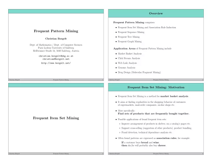
  66. Neural Spike Data: Selective Participation neurons neurons time time Association Rules • Both diagrams show the same (simulated) data, but on the right the 20 neurons of the assembly are collected at the bottom. • Only about 75% of the neurons (randomly chosen) participate in each synchronous firing. Hence there is no frequent item set comprising all of them. • Rather a frequent item set mining approach finds a large number of frequent item sets with 12 to 16 neurons. • Possible approach: fault-tolerant frequent item set mining . Christian Borgelt Frequent Pattern Mining 273 Christian Borgelt Frequent Pattern Mining 274 Association Rules: Basic Notions Association Rules: Formal Definition • Often found patterns are expressed as association rules , for example: Given: If a customer buys bread and wine , • a set B = { i 1 , . . . , i m } of items, then she/he will probably also buy cheese . • a tuple T = ( t 1 , . . . , t n ) of transactions over B , • Formally, we consider rules of the form X → Y , • a real number ς min , 0 < ς min ≤ 1, the minimum support , with X, Y ⊆ B and X ∩ Y = ∅ . • a real number c min , 0 < c min ≤ 1, the minimum confidence . • Support of a Rule X → Y : Desired: Either: ς T ( X → Y ) = σ T ( X ∪ Y ) (more common: rule is correct) • the set of all association rules , that is, the set Or: ς T ( X → Y ) = σ T ( X ) (more plausible: rule is applicable) R = { R : X → Y | ς T ( R ) ≥ ς min ∧ c T ( R ) ≥ c min } . • Confidence of a Rule X → Y : General Procedure: c T ( X → Y ) = σ T ( X ∪ Y ) = s T ( X ∪ Y ) = s T ( I ) σ T ( X ) s T ( X ) s T ( X ) • Find the frequent item sets. The confidence can be seen as an estimate of P ( Y | X ). • Construct rules and filter them w.r.t. ς min and c min . Christian Borgelt Frequent Pattern Mining 275 Christian Borgelt Frequent Pattern Mining 276

  67. Generating Association Rules Properties of the Confidence • Which minimum support has to be used for finding the frequent item sets • From ∀ I : ∀ J ⊆ I : s T ( I ) ≤ s T ( J ) it obviously follows depends on the definition of the support of a rule: s T ( X ∪ Y ) ≥ s T ( X ∪ Y ) ∀ X, Y : ∀ a ∈ X : ◦ If ς T ( X → Y ) = σ T ( X ∪ Y ), s T ( X ) s T ( X − { a } ) or equivalently s min = ⌈ nς min ⌉ . then σ min = ς min and therefore ◦ If ς T ( X → Y ) = σ T ( X ), ∀ X, Y : ∀ a ∈ X : c T ( X → Y ) ≥ c T ( X − { a } → Y ∪ { a } ) . then σ min = ς min c min or equivalently s min = ⌈ nς min c min ⌉ . That is: Moving an item from the antecedent to the consequent cannot increase the confidence of a rule. • After the frequent item sets have been found, the rule construction then traverses all frequent item sets I and • As an immediate consequence we have splits them into disjoint subsets X and Y ( X ∩ Y = ∅ and X ∪ Y = I ), thus forming rules X → Y . ∀ X, Y : ∀ a ∈ X : c T ( X → Y ) < c min → c T ( X − { a } → Y ∪ { a } ) < c min . ◦ Filtering rules w.r.t. confidence is always necessary. That is: If a rule fails to meet the minimum confidence, no rules over the same item set and with items moved ◦ Filtering rules w.r.t. support is only necessary if ς T ( X → Y ) = σ T ( X ). from antecedent to consequent need to be considered. Christian Borgelt Frequent Pattern Mining 277 Christian Borgelt Frequent Pattern Mining 278 Generating Association Rules Generating Association Rules function rules ( F ); ( ∗ — generate association rules ∗ ) function candidates ( F k ) ( ∗ generate candidates with k + 1 items ∗ ) R := ∅ ; ( ∗ initialize the set of rules ∗ ) begin forall f ∈ F do begin ( ∗ traverse the frequent item sets ∗ ) E := ∅ ; ( ∗ initialize the set of candidates ∗ ) m := 1; ( ∗ start with rule heads (consequents) ∗ ) forall f 1 , f 2 ∈ F k ( ∗ traverse all pairs of frequent item sets ∗ ) � H m := i ∈ f {{ i }} ; ( ∗ that contain only one item ∗ ) with f 1 = { a 1 , . . . , a k − 1 , a k } ( ∗ that differ only in one item and ∗ ) repeat ( ∗ traverse rule heads of increasing size ∗ ) f 2 = { a 1 , . . . , a k − 1 , a ′ and k } ( ∗ are in a lexicographic order ∗ ) forall h ∈ H m do ( ∗ traverse the possible rule heads ∗ ) a k < a ′ and k do begin ( ∗ (the order is arbitrary, but fixed) ∗ ) s T ( f ) if s T ( f − h ) ≥ c min ( ∗ if the confidence is high enough, ∗ ) f := f 1 ∪ f 2 = { a 1 , . . . , a k − 1 , a k , a ′ k } ; ( ∗ union has k + 1 items ∗ ) then R := R ∪ { [( f − h ) → h ] } ; ( ∗ add rule to the result ∗ ) if ∀ a ∈ f : f − { a } ∈ F k ( ∗ only if all subsets are frequent, ∗ ) else H m := H m − { h } ; ( ∗ otherwise discard the head ∗ ) then E := E ∪ { f } ; ( ∗ add the new item set to the candidates ∗ ) H m +1 := candidates( H m ); ( ∗ create heads with one item more ∗ ) m := m + 1; ( ∗ increment the head item counter ∗ ) end ; ( ∗ (otherwise it cannot be frequent) ∗ ) until H m = ∅ or m ≥ | f | ; ( ∗ until there are no more rule heads ∗ ) ( ∗ return the generated candidates ∗ ) return E ; end ; ( ∗ or antecedent would become empty ∗ ) end ( ∗ candidates ∗ ) return R ; ( ∗ return the rules found ∗ ) end ; ( ∗ rules ∗ ) Christian Borgelt Frequent Pattern Mining 279 Christian Borgelt Frequent Pattern Mining 280

  68. Frequent Item Sets: Example Generating Association Rules transaction database frequent item sets Example: I = { a, c, e } , X = { c, e } , Y = { a } . 1: { a, d, e } 0 items 1 item 2 items 3 items c T ( c, e → a ) = s T ( { a, c, e } ) = 3 2: { b, c, d } 4 = 75% ∅ : 10 { a } : 7 { a, c } : 4 { a, c, d } : 3 s T ( { c, e } ) 3: { a, c, e } { b } : 3 { a, d } : 5 { a, c, e } : 3 4: { a, c, d, e } { c } : 7 { a, e } : 6 { a, d, e } : 4 5: { a, e } { d } : 6 { b, c } : 3 Minimum confidence: 80% 6: { a, c, d } { e } : 7 { c, d } : 4 7: { b, c } { c, e } : 4 association support of support of confidence 8: { a, c, d, e } { d, e } : 4 rule all items antecedent 9: { c, b, e } b → c 3 (30%) 3 (30%) 100% 10: { a, d, e } d → a 5 (50%) 6 (60%) 83.3% e → a 6 (60%) 7 (70%) 85.7% • The minimum support is s min = 3 or σ min = 0 . 3 = 30% in this example. a → e 6 (60%) 7 (70%) 85.7% d, e → a 4 (40%) 4 (40%) 100% • There are 2 5 = 32 possible item sets over B = { a, b, c, d, e } . a, d → e 4 (40%) 5 (50%) 80% • There are 16 frequent item sets (but only 10 transactions). Christian Borgelt Frequent Pattern Mining 281 Christian Borgelt Frequent Pattern Mining 282 Support of an Association Rule Rules with Multiple Items in the Consequent? The two rule support definitions are not equivalent: • The general definition of association rules X → Y allows for multiple items in the consequent (i.e. | Y | ≥ 1). transaction database two association rules • However: If a → b, c is an association rule, 1: { a, c, e } association support of support of confidence then a → b and a → c are also association rules. 2: { b, d } rule all items antecedent 3: { b, c, d } Because: (regardless of the rule support definition) a → c 3 (37.5%) 5 (62.5%) 60.0% 4: { a, e } ς T ( a → b ) ≥ ς T ( a → b, c ), c T ( a → b ) ≥ c T ( a → b, c ), b → d 4 (50.0%) 4 (50.0%) 100.0% 5: { a, b, c, d } ς T ( a → c ) ≥ ς T ( a → b, c ), c T ( a → c ) ≥ c T ( a → b, c ). 6: { c, e } Let the minimum confidence be c min = 60%. • The two simpler rules are often sufficient (e.g. for product suggestions), 7: { a, b, d } 8: { a, c, d } even though they contain less information. ◦ a → b, c provides information about the joint conditional occurence of b and c (condition a ). • For ς T ( R ) = σ ( X ∪ Y ) and 3 / 8 < ς min ≤ 4 / 8 only the rule b → d is generated, but not the rule a → c . ◦ a → b and a → c only provide information about the individual conditional occurrences of b and c (condition a ). • For ς T ( R ) = σ ( X ) there is no value ς min that generates only the rule b → d , In most applications this additional information but not at the same time also the rule a → c . does not yield any additional benefit. Christian Borgelt Frequent Pattern Mining 283 Christian Borgelt Frequent Pattern Mining 284

  69. Rules with Multiple Items in the Consequent? Rule Extraction from Prefix Tree • If the rule support is defined as ς T ( X → Y ) = σ T ( X ∪ Y ), • Restriction to rules with one item in the head/consequent. we can go one step further in ruling out multi-item consequents. • Exploit the prefix tree to find the support of the body/antecedent. • If a → b, c is an association rule, • Traverse the item set tree breadth-first or depth-first. then a, b → c and a, c → b are also association rules. • For each node traverse the path to the root and Because: (confidence relationships always hold) generate and test one rule per node. ς T ( a, b → c ) ≥ ς T ( a → b, c ), c T ( a, b → c ) ≥ c T ( a → b, c ), ς T ( a, c → b ) ≥ ς T ( a → b, c ), c T ( a, c → b ) ≥ c T ( a → b, c ). root ✡ • First rule: Get the support of the body/ ✡ • Together with a → b and a → c , the rules a, b → c and a, c → b ♣♣♣♣♣ antecedent from the parent node. contain effectively the same information as the rule a → b, c , ✡ ✡ although in a different form. hdnode • Next rules: Discard the head/conse- ✲ ✡ ❏ j head i ✡ ❏ ♣ ♣ ♣ quent item from the downward path ♣ prev ♣ • For example, product suggestions can be made by first applying a → b , ✸ ✑ ✑✑✑ ✡ ❏ j and follow the remaining path from the ✡ ❏ ♣♣♣♣♣ same hypothetically assuming that b is actually added to the shopping cart, ✛ body path current node. and then applying a, b → c to suggest both b and c . ✡ ✡ isnode Christian Borgelt Frequent Pattern Mining 285 Christian Borgelt Frequent Pattern Mining 286 Reminder: Prefix Tree Additional Rule Filtering: Simple Measures ˆ • General idea: Compare P T ( Y | X ) = c T ( X → Y ) a b c d e a d ˆ = c T ( ∅ → Y ) = σ T ( Y ). c and P T ( Y ) b ab ac ad ae bc bd be cd ce de • (Absolute) confidence difference to prior: b c c d d d d T ( R ) = | c T ( X → Y ) − σ T ( Y ) | abc abd abe acd ace ade bcd bce bde cde c d d d • Lift value: l T ( R ) = c T ( X → Y ) abcd abce abde acde bcde σ T ( Y ) d abcde A (full) prefix tree for the five items a, b, c, d, e . • (Absolute) difference of lift value to 1: � � c T ( X → Y ) � � • Based on a global order of the items (which can be arbitrary). q T ( R ) = � − 1 � � � σ T ( Y ) � � • The item sets counted in a node consist of • (Absolute) difference of lift quotient to 1: ◦ all items labeling the edges to the node (common prefix) and � � c T ( X → Y ) �� σ T ( Y ) � � r T ( R ) = � � 1 − min , � ◦ one item following the last edge label in the item order. � � σ T ( Y ) c T ( X → Y ) � Christian Borgelt Frequent Pattern Mining 287 Christian Borgelt Frequent Pattern Mining 288

  70. Additional Rule Filtering: More Sophisticated Measures An Information-theoretic Evaluation Measure • Consider the 2 × 2 contingency table or the estimated probability table: Information Gain (Kullback and Leibler 1951, Quinlan 1986) n X �⊆ t X ⊆ t X �⊆ t X ⊆ t � Based on Shannon Entropy H = − p i log 2 p i (Shannon 1948) Y �⊆ t n 00 n 01 n 0 . Y �⊆ t p 00 p 01 p 0 . i =1 Y ⊆ t n 10 n 11 n 1 . Y ⊆ t p 10 p 11 p 1 . n . 0 n . 1 n .. p . 0 p . 1 1 I gain ( X, Y ) = H ( Y ) − H ( Y | X ) � �� � � �� � • n .. is the total number of transactions.   k Y k X k Y � � � = − p i. log 2 p i. − p .j  − p i | j log 2 p i | j n . 1 is the number of transactions to which the rule is applicable.  n 11 is the number of transactions for which the rule is correct. i =1 j =1 i =1 p ij = n ij p .j = n .j p i. = n i. It is n .. , n .. , for i, j = 1 , 2. n .. H ( Y ) Entropy of the distribution of Y H ( Y | X ) Expected entropy of the distribution of Y • General idea: Use measures for the strength of dependence of X and Y . if the value of the X becomes known • There is a large number of such measures of dependence H ( Y ) − H ( Y | X ) Expected entropy reduction or information gain originating from statistics, decision tree induction etc. Christian Borgelt Frequent Pattern Mining 289 Christian Borgelt Frequent Pattern Mining 290 Interpretation of Shannon Entropy Question/Coding Schemes • Let S = { s 1 , . . . , s n } be a finite set of alternatives P ( s 1 ) = 0 . 10 , P ( s 2 ) = 0 . 15 , P ( s 3 ) = 0 . 16 , P ( s 4 ) = 0 . 19 , P ( s 5 ) = 0 . 40 � n having positive probabilities P ( s i ), i = 1 , . . . , n , satisfying i =1 P ( s i ) = 1. � Shannon entropy: − i P ( s i ) log 2 P ( s i ) = 2 . 15 bit/symbol • Shannon Entropy: Linear Traversal Equal Size Subsets n � H ( S ) = − P ( s i ) log 2 P ( s i ) s 1 , s 2 , s 3 , s 4 , s 5 s 1 , s 2 , s 3 , s 4 , s 5 i =1 s 2 , s 3 , s 4 , s 5 0.25 0.75 s 1 , s 2 s 3 , s 4 , s 5 • Intuitively: Expected number of yes/no questions that have s 3 , s 4 , s 5 to be asked in order to determine the obtaining alternative. 0.59 s 4 , s 5 s 4 , s 5 ◦ Suppose there is an oracle, which knows the obtaining alternative, but responds only if the question can be answered with “yes” or “no”. 0.10 0.15 0.16 0.19 0.40 0.10 0.15 0.16 0.19 0.40 s 1 s 2 s 3 s 4 s 5 s 1 s 2 s 3 s 4 s 5 ◦ A better question scheme than asking for one alternative after the other 1 2 3 4 4 2 2 2 3 3 can easily be found: Divide the set into two subsets of about equal size. Code length: 3.24 bit/symbol Code length: 2.59 bit/symbol ◦ Ask for containment in an arbitrarily chosen subset. Code efficiency: 0.664 Code efficiency: 0.830 ◦ Apply this scheme recursively → number of questions bounded by ⌈ log 2 n ⌉ . Christian Borgelt Frequent Pattern Mining 291 Christian Borgelt Frequent Pattern Mining 292

  71. Question/Coding Schemes Question/Coding Schemes • Splitting into subsets of about equal size can lead to a bad arrangement P ( s 1 ) = 0 . 10 , P ( s 2 ) = 0 . 15 , P ( s 3 ) = 0 . 16 , P ( s 4 ) = 0 . 19 , P ( s 5 ) = 0 . 40 of the alternatives into subsets → high expected number of questions. � Shannon entropy: − i P ( s i ) log 2 P ( s i ) = 2 . 15 bit/symbol • Good question schemes take the probability of the alternatives into account. Shannon–Fano Coding (1948) Huffman Coding (1952) • Shannon-Fano Coding (1948) s 1 , s 2 , s 3 , s 4 , s 5 s 1 , s 2 , s 3 , s 4 , s 5 ◦ Build the question/coding scheme top-down. 0.41 0.59 0.60 s 1 , s 2 , s 3 s 4 , s 5 s 1 , s 2 , s 3 , s 4 ◦ Sort the alternatives w.r.t. their probabilities. 0.25 0.25 0.35 ◦ Split the set so that the subsets have about equal probability s 1 , s 2 s 1 , s 2 s 3 , s 4 (splits must respect the probability order of the alternatives). 0.10 0.15 0.16 0.19 0.40 0.10 0.15 0.16 0.19 0.40 s 1 s 2 s 3 s 4 s 5 s 1 s 2 s 3 s 4 s 5 • Huffman Coding (1952) 3 3 2 2 2 3 3 3 3 1 ◦ Build the question/coding scheme bottom-up. Code length: 2.25 bit/symbol Code length: 2.20 bit/symbol ◦ Start with one element sets. Code efficiency: 0.955 Code efficiency: 0.977 ◦ Always combine those two sets that have the smallest probabilities. Christian Borgelt Frequent Pattern Mining 293 Christian Borgelt Frequent Pattern Mining 294 Question/Coding Schemes Interpretation of Shannon Entropy • It can be shown that Huffman coding is optimal P ( s 1 ) = 1 P ( s 2 ) = 1 P ( s 3 ) = 1 P ( s 4 ) = 1 P ( s 5 ) = 1 2 , 4 , 8 , 16 , 16 if we have to determine the obtaining alternative in a single instance. � Shannon entropy: − i P ( s i ) log 2 P ( s i ) = 1 . 875 bit/symbol (No question/coding scheme has a smaller expected number of questions.) If the probability distribution allows for a Perfect Question Scheme • Only if the obtaining alternative has to be determined in a sequence perfect Huffman code (code efficiency 1), s 1 , s 2 , s 3 , s 4 , s 5 of (independent) situations, this scheme can be improved upon. the Shannon entropy can easily be inter- preted as follows: s 2 , s 3 , s 4 , s 5 • Idea: Process the sequence not instance by instance, � but combine two, three or more consecutive instances and − P ( s i ) log 2 P ( s i ) s 3 , s 4 , s 5 ask directly for the obtaining combination of alternatives. i 1 s 4 , s 5 � · log 2 = P ( s i ) . • Although this enlarges the question/coding scheme, the expected number P ( s i ) 1 1 1 1 1 i 2 4 8 16 16 � �� � � �� � s 1 s 2 s 3 s 4 s 5 of questions per identification is reduced (because each interrogation occurrence path length 1 2 3 4 4 identifies the obtaining alternative for several situations). in tree probability Code length: 1.875 bit/symbol In other words, it is the expected number • However, the expected number of questions per identification of needed yes/no questions. Code efficiency: 1 of an obtaining alternative cannot be made arbitrarily small. Shannon showed that there is a lower bound, namely the Shannon entropy. Christian Borgelt Frequent Pattern Mining 295 Christian Borgelt Frequent Pattern Mining 296

  72. A Statistical Evaluation Measure A Statistical Evaluation Measure χ 2 Measure χ 2 Measure • Compares the actual joint distribution • Compares the actual joint distribution with a hypothetical independent distribution . with a hypothetical independent distribution . • Uses absolute comparison. • Uses absolute comparison. • Can be interpreted as a difference measure. • Can be interpreted as a difference measure. k X k Y k X k Y ( p i. p .j − p ij ) 2 ( p i. p .j − p ij ) 2 � � � � χ 2 ( X, Y ) = χ 2 ( X, Y ) = n .. n .. p i. p .j p i. p .j i =1 j =1 i =1 j =1 • For k X = k Y = 2 (as for rule evaluation) the χ 2 measure simplifies to • Side remark: Information gain can also be interpreted as a difference measure. ( p 1 . p . 1 − p 11 ) 2 ( n 1 . n . 1 − n .. n 11 ) 2 k X k Y p ij χ 2 ( X, Y ) = n .. � � p 1 . (1 − p 1 . ) p . 1 (1 − p . 1 ) = n .. n 1 . ( n .. − n 1 . ) n . 1 ( n .. − n . 1 ) . I gain ( X, Y ) = p ij log 2 p i. p .j j =1 i =1 Christian Borgelt Frequent Pattern Mining 297 Christian Borgelt Frequent Pattern Mining 298 Examples from the Census Data Examples from the Census Data All rules are stated as salary>50K <- education=Masters (5.4, 54.9, 2.29) salary>50K <- occupation=Exec-managerial (12.5, 47.8, 2.00) consequent <- antecedent (support%, confidence%, lift) salary>50K <- relationship=Wife (4.8, 46.9, 1.96) where the support of a rule is the support of the antecedent. salary>50K <- occupation=Prof-specialty (12.6, 45.1, 1.89) salary>50K <- relationship=Husband (40.4, 44.9, 1.88) Trivial/Obvious Rules salary>50K <- marital=Married-civ-spouse (45.8, 44.6, 1.86) edu_num=13 <- education=Bachelors (16.4, 100.0, 6.09) salary>50K <- education=Bachelors (16.4, 41.3, 1.73) sex=Male <- relationship=Husband (40.4, 99.99, 1.50) salary>50K <- hours=overtime (26.0, 40.6, 1.70) sex=Female <- relationship=Wife (4.8, 99.9, 3.01) salary>50K <- occupation=Exec-managerial hours=overtime Interesting Comparisons (5.5, 60.1, 2.51) salary>50K <- occupation=Prof-specialty hours=overtime marital=Never-married <- age=young sex=Female (12.3, 80.8, 2.45) (4.4, 57.3, 2.39) marital=Never-married <- age=young sex=Male (17.4, 69.9, 2.12) salary>50K <- education=Bachelors hours=overtime salary>50K <- occupation=Exec-managerial sex=Male (8.9, 57.3, 2.40) (6.0, 54.8, 2.29) salary>50K <- occupation=Exec-managerial (12.5, 47.8, 2.00) salary>50K <- education=Masters (5.4, 54.9, 2.29) hours=overtime <- education=Masters (5.4, 41.0, 1.58) Christian Borgelt Frequent Pattern Mining 299 Christian Borgelt Frequent Pattern Mining 300

  73. Examples from the Census Data Examples from the Census Data salary>50K <- occupation=Prof-specialty hours=half-time <- occupation=Other-service age=young marital=Married-civ-spouse (6.5, 70.8, 2.96) (4.4, 37.2, 3.08) salary>50K <- occupation=Exec-managerial hours=overtime <- salary>50K (23.9, 44.0, 1.70) marital=Married-civ-spouse (7.4, 68.1, 2.85) hours=overtime <- occupation=Exec-managerial (12.5, 43.8, 1.69) hours=overtime <- occupation=Exec-managerial salary>50K salary>50K <- education=Bachelors (6.0, 55.1, 2.12) marital=Married-civ-spouse (8.5, 67.2, 2.81) hours=overtime <- education=Masters (5.4, 40.9, 1.58) salary>50K <- hours=overtime education=Bachelors <- occupation=Prof-specialty marital=Married-civ-spouse (15.6, 56.4, 2.36) (12.6, 36.2, 2.20) education=Bachelors <- occupation=Exec-managerial marital=Married-civ-spouse <- salary>50K (23.9, 85.4, 1.86) (12.5, 33.3, 2.03) education=HS-grad <- occupation=Transport-moving (4.8, 51.9, 1.61) education=HS-grad <- occupation=Machine-op-inspct (6.2, 50.7, 1.6) Christian Borgelt Frequent Pattern Mining 301 Christian Borgelt Frequent Pattern Mining 302 Examples from the Census Data Summary Association Rules occupation=Prof-specialty <- education=Masters • Association Rule Induction is a Two Step Process (5.4, 49.0, 3.88) ◦ Find the frequent item sets (minimum support). occupation=Prof-specialty <- education=Bachelors sex=Female ◦ Form the relevant association rules (minimum confidence). (5.1, 34.7, 2.74) occupation=Adm-clerical <- education=Some-college sex=Female (8.6, 31.1, 2.71) • Generating the Association Rules ◦ Form all possible association rules from the frequent item sets. sex=Female <- occupation=Adm-clerical (11.5, 67.2, 2.03) sex=Female <- occupation=Other-service (10.1, 54.8, 1.65) ◦ Filter “interesting” association rules sex=Female <- hours=half-time (12.1, 53.7, 1.62) based on minimum support and minimum confidence. age=young <- hours=half-time (12.1, 53.3, 1.79) • Filtering the Association Rules age=young <- occupation=Handlers-cleaners (4.2, 50.6, 1.70) ◦ Compare rule confidence and consequent support. age=senior <- workclass=Self-emp-not-inc (7.9, 31.1, 1.57) ◦ Information gain, χ 2 measure ◦ In principle: other measures used for decision tree induction. Christian Borgelt Frequent Pattern Mining 303 Christian Borgelt Frequent Pattern Mining 304

  74. Mining More Complex Patterns • The search scheme in Frequent Graph/Tree/Sequence mining is the same, namely the general scheme of searching with a canonical form. • Frequent (Sub)Graph Mining comprises the other areas: ◦ Trees are special graphs, namely graphs that are singly connected. ◦ Sequences can be seen as special trees, namely chains (only one or two branches — depending on the choice of the root). Mining More Complex Patterns • Frequent Sequence Mining and Frequent Tree Mining can exploit: ◦ Specialized canonical forms that allow for more efficient checks. ◦ Special data structures to represent the database to mine, so that support counting becomes more efficient. • We will treat Frequent (Sub)Graph Mining first and will discuss optimizations for the other areas later. Christian Borgelt Frequent Pattern Mining 305 Christian Borgelt Frequent Pattern Mining 306 Search Space Comparison Search Space Comparison Search space for sets: (5 items) Search space for sequences: (4 items, no repetitions) a c b d a b c d e a b c d e c a c a a c b d d b d b c c c a a c a a c a c a ab ac ad ae bc bd be cd ce de ab ac ad ae bc bd be cd ce de d b d b d d b d d b b b c c c a c a a a c c a a d d b b d d d b d b b b abc abd abe acd ace ade bcd bce bde cde abc abd abe acd ace ade bcd bce bde cde • Red part corresponds to search space for sets. abcd abce abde acde bcde abcd abce abde acde bcde • The search space for (sub)sequences is considerably larger than the one for sets. abcde abcde • However: support of (sub)sequences reduces much faster with increasing length. Search space for sequences: (5 items, no repetitions) ◦ Out of k items only one set can be formed, but k ! sequences (every order yields a different sequences). a b c d e b c d e a c d e a b d e a b c e a b c d c e e c e c c e a e a c e a c e a e a e a c e a c e a e a c c a c a a c d b d b b d d d d b d d b b d b b b b d d b d b ◦ All k ! sequences cover the set (tendency towards higher support). d e c e c d d e b e b d c e b e b c c d b d b c d e c e c d d e a e a d c e a e a c c d a d a c d e b e b d d e a e a d b e a e a b b d a d a b c e b e b c c e a e a c b e a e a b b c a c a b c d b d b c c d a d a c b d a d a b b c a c a b e d e c d c e d e b d b e c e b c b d c d b c b e d e c d c e d e a d a e c e a c a d c d a c a e d e b d b e d e a d a e b e a b a d b d a b a e c e b c b e c e a c a e b e a b a c b c a b a d c d b c b d c d a c a d b d a b a c b c a b a ◦ To cover a specific sequence, a specific order is required. • Red part corresponds to search space for sets (top right). (tendency towards lower support). Christian Borgelt Frequent Pattern Mining 307 Christian Borgelt Frequent Pattern Mining 308

  75. Molecular Fragment Mining • Motivation: Accelerating Drug Development ◦ Phases of drug development: pre-clinical and clinical ◦ Data gathering by high-throughput screening: building molecular databases with activity information ◦ Acceleration potential by intelligent data analysis: Motivation: (quantitative) structure-activity relationship discovery Molecular Fragment Mining • Mining Molecular Databases ◦ Example data: NCI DTP HIV Antiviral Screen data set ◦ Description languages for molecules: SMILES, SLN, SDfile/Ctab etc. ◦ Finding common molecular substructures ◦ Finding discriminative molecular substructures Christian Borgelt Frequent Pattern Mining 309 Christian Borgelt Frequent Pattern Mining 310 Accelerating Drug Development Phases of Drug Development • Developing a new drug can take 10 to 12 years • Discovery and Optimization of Candidate Substances (from the choice of the target to the introduction into the market). ◦ High-Throughput Screening • In recent years the duration of the drug development processes increased ◦ Lead Discovery and Lead Optimization continuously; at the same the number of substances under development has gone down drastically. • Pre-clinical Test Series (tests with animals, ca. 3 years) ◦ Fundamental test w.r.t. effectiveness and side effects • Due to high investments pharmaceutical companies must secure their market position and competitiveness by only a few, highly successful drugs . • Clinical Test Series (tests with humans, ca. 4–6 years) • As a consequence the chances for the development ◦ Phase 1: ca. 30–80 healthy humans of drugs for target groups Check for side effects ◦ with rare diseases or ◦ Phase 2: ca. 100–300 humans exhibiting the symptoms of the target disease Check for effectiveness ◦ with special diseases in developing countries ◦ Phase 3: up to 3000 healthy and ill humans at least 3 years are considerably reduced. Detailed check of effectiveness and side effects • A significant reduction of the development time could mitigate this trend • Official Acceptance as a Drug or even reverse it. (Source: Bundesministerium f¨ ur Bildung und Forschung, Germany) Christian Borgelt Frequent Pattern Mining 311 Christian Borgelt Frequent Pattern Mining 312

  76. Drug Development: Acceleration Potential High-Throughput Screening • The length of the pre-clinical and clinical tests series can hardly be reduced, On so-called micro-plates proteins/cells are automatically combined with a large since they serve the purpose to ensure the safety of the patients. variety of chemical compounds. • Therefore approaches to speed up the development process pictures not available in online version usually target the pre-clinical phase before the animal tests. • In particular, it is tried to improve the search for new drug candidates ( lead discovery ) and their optimization ( lead optimization ). Here Frequent Pattern Mining can help. One possible approach: • With high-throughput screening a very large number of substances is tested automatically and their activity is determined. • The resulting molecular databases are analyzed by trying to find common substructures of active substances. Christian Borgelt Frequent Pattern Mining 313 Christian Borgelt Frequent Pattern Mining 314 High-Throughput Screening High-Throughput Screening The filled micro-plates are then evaluated in spectrometers After the measurement the substances are classified as active or inactive . (w.r.t. absorption, fluorescence, luminescence, polarization etc). By analyzing the results one tries to understand the dependencies pictures not available in online version between molecular structure and activity. QSAR — Quantitative Structure-Activity Relationship Modeling picture not available in online version In this area a large number of data mining algorithms are used: • frequent pattern mining • feature selection methods • decision trees • neural networks etc. Christian Borgelt Frequent Pattern Mining 315 Christian Borgelt Frequent Pattern Mining 316

  77. Example: NCI DTP HIV Antiviral Screen Form of the Input Data • Among other data sets, the National Cancer Institute (NCI) has made Excerpt from the NCI DTP HIV Antiviral Screen data set (SMILES format): the DTP HIV Antiviral Screen Data Set publicly available. 737, 0,CN(C)C1=[S+][Zn]2(S1)SC(=[S+]2)N(C)C 2018, 0,N#CC(=CC1=CC=CC=C1)C2=CC=CC=C2 • A large number of chemical compounds where tested 19110,0,OC1=C2N=C(NC3=CC=CC=C3)SC2=NC=N1 whether they protect human CEM cells against an HIV-1 infection. 20625,2,NC(=N)NC1=C(SSC2=C(NC(N)=N)C=CC=C2)C=CC=C1.OS(O)(=O)=O 22318,0,CCCCN(CCCC)C1=[S+][Cu]2(S1)SC(=[S+]2)N(CCCC)CCCC • Substances that provided 50% protection were retested. 24479,0,C[N+](C)(C)C1=CC2=C(NC3=CC=CC=C3S2)N=N1 50848,2,CC1=C2C=CC=CC2=N[C-](CSC3=CC=CC=C3)[N+]1=O • Substances that reproducibly provided 100% protection 51342,0,OC1=C2C=NC(=NC2=C(O)N=N1)NC3=CC=C(Cl)C=C3 are listed as “confirmed active” (CA) . 55721,0,NC1=NC(=C(N=O)C(=N1)O)NC2=CC(=C(Cl)C=C2)Cl 55917,0,O=C(N1CCCC[CH]1C2=CC=CN=C2)C3=CC=CC=C3 • Substances that reproducibly provided at least 50% protection 64054,2,CC1=C(SC[C-]2N=C3C=CC=CC3=C(C)[N+]2=O)C=CC=C1 are listed as “moderately active” (CM) . 64055,1,CC1=CC=CC(=C1)SC[C-]2N=C3C=CC=CC3=C(C)[N+]2=O 64057,2,CC1=C2C=CC=CC2=N[C-](CSC3=NC4=CC=CC=C4S3)[N+]1=O • All other substances 66151,0,[O-][N+](=O)C1=CC2=C(C=NN=C2C=C1)N3CC3 are listed as “confirmed inactive” (CI) . ... • 325 CA , 877 CM , 35 969 CI (total: 37 171 substances) identification number, activity (2: CA, 1: CM, 0: CI), molecule description in SMILES notation Christian Borgelt Frequent Pattern Mining 317 Christian Borgelt Frequent Pattern Mining 318 Input Format: SMILES Notation and SLN Input Format: Grammar for SMILES and SLN SMILES Notation: (e.g. Daylight, Inc.) General grammar for (linear) molecule descriptions (SMILES and SLN): c1:c:c(-F):c:c2:c:1-C1-C(-C-C-2)-C2-C(-C)(-C-C-1)-C(-O)-C-C-2 Molecule ::= Atom Branch Branch ::= ε SLN (SYBYL Line Notation): (Tripos, Inc.) | Bond Atom Branch | Bond Label Branch black: non-terminal symbols C[1]H:CH:C(F):CH:C[8]:C:@1-C[10]H-CH(-CH2-CH2-@8)-C[20]H-C(-CH3) | ( Branch ) Branch blue : terminal symbols (-CH2-CH2-@10)-CH(-CH2-CH2-@20)-OH Atom ::= Element LabelDef LabelDef ::= ε | Label LabelDef Represented Molecule: Full Representation Simplified Representation The definitions of the non-terminals ”Element”, ”Bond”, and ”Label” depend on the chosen description language. For SMILES it is: H H H H H H H H H C C H C C C H Element ::= B | C | N | O | F | [H] | [He] | [Li] | [Be] | . . . H O F C C C C C C C C O F Bond ::= ε | - | = | # | : | . C C C C H C Label ::= Digit | % Digit Digit C C C H H H H H H Digit ::= 0 | 1 | . . . | 9 H H H H Christian Borgelt Frequent Pattern Mining 319 Christian Borgelt Frequent Pattern Mining 320

  78. Input Format: SDfile/Ctab Finding Common Molecular Substructures Some Molecules from the NCI HIV Database L-Alanine (13C) user initials, program, date/time etc. O comment N 6 5 0 0 1 0 3 V2000 O O N -0.6622 0.5342 0.0000 C 0 0 2 0 0 0 N O N O N C 1 N 4 3 N 0.6622 -0.3000 0.0000 C 0 0 0 0 0 0 N O C O -0.7207 2.0817 0.0000 C 1 0 0 0 0 0 N O N O C -1.8622 -0.3695 0.0000 N 0 3 0 0 0 0 O O N N N O 2 O 6 5 O O O P 0.6220 -1.8037 0.0000 O 0 0 0 0 0 0 O O O O N N N 1.9464 0.4244 0.0000 O 0 5 0 0 0 0 O N N N 1 2 1 0 0 0 O O 1 3 1 1 0 0 O Common Fragment 1 4 1 0 0 0 N 2 5 2 0 0 0 O N O SDfile: Structure-data file 2 6 1 0 0 0 M END N Ctab: Connection table (lines 4–16) O > <value> O N O ➞ Elsevier Science O O O N N N 0.2 O O O $$$$ O N N N Christian Borgelt Frequent Pattern Mining 321 Christian Borgelt Frequent Pattern Mining 322 Finding Molecular Substructures • Common Molecular Substructures ◦ Analyze only the active molecules. ◦ Find molecular fragments that appear frequently in the molecules. • Discriminative Molecular Substructures ◦ Analyze the active and the inactive molecules. Frequent (Sub)Graph Mining ◦ Find molecular fragments that appear frequently in the active molecules and only rarely in the inactive molecules. • Rationale in both cases : ◦ The found fragments can give hints which structural properties are responsible for the activity of a molecule. ◦ This can help to identify drug candidates (so-called pharmacophores ) and to guide future screening efforts. Christian Borgelt Frequent Pattern Mining 323 Christian Borgelt Frequent Pattern Mining 324

  79. Frequent (Sub)Graph Mining: General Approach Frequent (Sub)Graph Mining: Basic Notions • Finding frequent item sets means to find • Let A = { a 1 , . . . , a m } be a set of attributes or labels . sets of items that are contained in many transactions . • A labeled or attributed graph is a triplet G = ( V, E, ℓ ), where • Finding frequent substructures means to find ◦ V is the set of vertices, graph fragments that are contained in many graphs ◦ E ⊆ V × V − { ( v, v ) | v ∈ V } is the set of edges, and in a given database of attributed graphs (user specifies minimum support). ◦ ℓ : V ∪ E → A assigns labels from the set A to vertices and edges. • Graph structure of vertices and edges has to be taken into account. Note that G is undirected and simple and contains no loops . However, graphs without these restrictions could be handled as well. ⇒ Search partially ordered set of graph structures instead of subsets. Note also that several vertices and edges may have the same attribute/label. Main problem: How can we avoid redundant search? Example: molecule representation • Usually the search is restricted to connected substructures . ◦ Connected substructures suffice for most applications. • Atom attributes: atom type (chemical element), charge, aromatic ring flag ◦ This restriction considerably narrows the search space. • Bond attributes: bond type (single, double, triple, aromatic) Christian Borgelt Frequent Pattern Mining 325 Christian Borgelt Frequent Pattern Mining 326 Frequent (Sub)Graph Mining: Basic Notions Frequent (Sub)Graph Mining: Basic Notions Note that for labeled graphs the same notions can be used as for normal graphs. Note that for labeled graphs the same notions can be used as for normal graphs. Without formal definition, we will use, for example: Without formal definition, we will use, for example: • A vertex v is incident to an edge e , and the edge is incident to the vertex v , • A vertex of a graph is called isolated if it is not incident to any edge. iff e = ( v, v ′ ) or e = ( v ′ , v ). • A vertex of a graph is called a leaf if it is incident to exactly one edge. • Two different vertices are adjacent or connected • An edge of a graph is called a bridge if removing it if they are incident to the same edge. increases the number of connected components of the graph. • A path is a sequence of edges connecting two vertices. More intuitively: a bridge is the only connection between two vertices, It is usually understood that no edge (and no vertex) occurs twice. that is, there is no other path on which one can reach the one from the other. • A graph is called connected if there exists a path between any two vertices. • An edge of a graph is called a leaf bridge if it is a bridge and incident to at least one leaf. • A subgraph consists of a subset of the vertices and a subset of the edges. If S is a (proper) subgraph of G we write S ⊆ G or S ⊂ G , respectively. In other words: an edge is a leaf bridge if removing it creates an isolated vertex. • A connected component of a graph is a subgraph that is connected and • All other bridges are called proper bridges . maximal in the sense that any larger subgraph containing it is not connected. Christian Borgelt Frequent Pattern Mining 327 Christian Borgelt Frequent Pattern Mining 328

  80. Frequent (Sub)Graph Mining: Basic Notions Frequent (Sub)Graph Mining: Basic Notions • Let G = ( V G , E G , ℓ G ) and S = ( V S , E S , ℓ S ) be two labeled graphs. Let S and G be two labeled graphs. A subgraph isomorphism of S to G or an occurrence of S in G • S and G are called isomorphic , written S ≡ G , iff S ⊑ G and G ⊑ S . is an injective function f : V S → V G with In this case a function f mapping S to G is called a graph isomorphism . ◦ ∀ v ∈ V S : ℓ S ( v ) = ℓ G ( f ( v )) and A function f mapping S to itself is called a graph automorphism . ◦ ∀ ( u, v ) ∈ E S : ( f ( u ) , f ( v )) ∈ E G ∧ ℓ S (( u, v )) = ℓ G (( f ( u ) , f ( v ))). • S is properly contained in G , written S ❁ G , iff S ⊑ G and S �≡ G . That is, the mapping f preserves the connection structure and the labels. • If S ⊑ G or S ❁ G , then there exists a (proper) subgraph G ′ of G , If such a mapping f exists, we write S ⊑ G (note the difference to S ⊆ G ). (that is, G ′ ⊆ G or G ′ ⊂ G , respectively), such that S and G ′ are isomorphic. This explains the term “subgraph isomorphism”. • Note that there may be several ways to map a labeled graph S to a labeled graph G so that the connection structure and the vertex and edge labels are preserved. • The set of all connected subgraphs of G is denoted by C ( G ). It may even be that the graph S can be mapped in several different ways to the It is obvious that for all S ∈ C ( G ) : S ⊑ G . same subgraph of G . This is the case if there exists a subgraph isomorphism of S However, there are (unconnected) graphs S with S ⊑ G that are not in C ( G ). to itself (a so-called graph automorphism ) that is not the identity. The set of all (connected) subgraphs is analogous to the power set of a set. Christian Borgelt Frequent Pattern Mining 329 Christian Borgelt Frequent Pattern Mining 330 Subgraph Isomorphism: Examples Subgraph Isomorphism: Examples N N S 2 S 2 O O S 1 S 1 N N f 2 : V S 2 → V G O O f 1 : V S 1 → V G N N O O O N O O O N O O G G • A molecule G that represents a graph in a database • The mapping must preserve the connection structure: and two graphs S 1 and S 2 that are contained in G . ∀ ( u, v ) ∈ E S : ( f ( u ) , f ( v )) ∈ E G . • The subgraph relationship is formally described by a mapping f • The mapping must preserve vertex and edge labels: of the vertices of one graph to the vertices of another: ∀ v ∈ V S : ℓ S ( v ) = ℓ G ( f ( v )) , ∀ ( u, v ) ∈ E S : ℓ S (( u, v )) = ℓ G (( f ( u ) , f ( v ))) . G = ( V G , E G ) , S = ( V S , E S ) , f : V S → V G . Here: oxygen must be mapped to oxygen, single bonds to single bonds etc. • This mapping must preserve the connection structure and the labels. Christian Borgelt Frequent Pattern Mining 331 Christian Borgelt Frequent Pattern Mining 332

  81. Subgraph Isomorphism: Examples Subgraph Isomorphism: Examples N N O S 2 S 3 O S 1 S 1 O N N f 2 : V S 2 → V G f 3 : V S 3 → V G g 2 : V S 2 → V G g 3 : V S 3 → V G O O f 1 : V S 1 → V G f 1 : V S 1 → V G N N O O O N O O O N O O G G • There may be more than one possible mapping / occurrence. • A graph may be mapped to itself ( automorphism ). (There are even three more occurrences of S 2 .) • Trivially, every graph possesses the identity as an automorphism. • However, we are currently only interested in whether there exists a mapping. (Every graph can be mapped to itself by mapping each vertex to itself.) (The number of occurrences will become important • If a graph (fragment) possesses an automorphism that is not the identity when we consider mining frequent (sub)graphs in a single graph.) there is more than one occurrence at the same location in another graph. • Testing whether a subgraph isomorphism exists between given graphs S and G • The number of occurrences of a graph (fragment) in a graph can be huge. is NP-complete (that is, requires exponential time unless P = NP). Christian Borgelt Frequent Pattern Mining 333 Christian Borgelt Frequent Pattern Mining 334 Frequent (Sub)Graph Mining: Basic Notions Frequent (Sub)Graph Mining: Formal Definition Let S be a labeled graph and G a tuple of labeled graphs. Given: • a set A = { a 1 , . . . , a m } of attributes or labels, • A labeled graph G ∈ G covers the labeled graph S or the labeled graph S is contained in a labeled graph G ∈ G iff S ⊑ G . • a tuple G = ( G 1 , . . . , G n ) of graphs with labels in A , • a number s min ∈ I N, 1 ≤ s min ≤ n , or (equivalently) • The set K G ( S ) = { k ∈{ 1 , . . . , n } | S ⊑ G k } is called the cover of S w.r.t. G . a number σ min ∈ I R, 0 < σ min ≤ 1, the minimum support . The cover of a graph is the index set of the database graphs that cover it. It may also be defined as a tuple of all labeled graphs that cover it Desired: (which, however, is complicated to write in formally correct way). • the set of frequent (sub)graphs or frequent fragments , that is, the set F G ( s min ) = { S | s G ( S ) ≥ s min } or (equivalently) • The value s G ( S ) = | K G ( S ) | is called the (absolute) support of S w.r.t. G . the set Φ G ( σ min ) = { S | σ G ( S ) ≥ σ min } . The value σ G ( S ) = 1 n | K G ( S ) | is called the relative support of S w.r.t. G . The support of S is the number or fraction of labeled graphs that contain it. σ min = 1 Note that with the relations s min = ⌈ nσ min ⌉ and n s min Sometimes σ G ( S ) is also called the (relative) frequency of S w.r.t. G . the two versions can easily be transformed into each other. Christian Borgelt Frequent Pattern Mining 335 Christian Borgelt Frequent Pattern Mining 336

  82. Frequent (Sub)Graphs: Example Properties of the Support of (Sub)Graphs • A brute force approach that enumerates all possible (sub)graphs, determines example molecules frequent molecular fragments ( s min = 2) their support, and discards infrequent (sub)graphs is usually infeasible : (graph database) ∗ (empty graph) The number of possible (connected) (sub)graphs, 3 S C N C grows very quickly with the number of vertices and edges. O S O C N • Idea: Consider the properties of a (sub)graph’s cover and support, in particular: 3 3 3 3 O S C N ∀ S : ∀ R ⊇ S : K G ( R ) ⊆ K G ( S ) . F O S S C C O C N 2 3 2 3 This property holds, because ∀ G : ∀ S : ∀ R ⊇ S : R ⊑ G → S ⊑ G . O S C N Each additional edge is another condition a database graph has to satisfy. O O S C S C N S C O N C O Graphs that do not satisfy this condition are removed from the cover. 2 3 2 2 • It follows: ∀ S : ∀ R ⊇ S : s G ( R ) ≤ s G ( S ) . O S C S C N The numbers N O below the subgraphs That is: If a (sub)graph is extended, its support cannot increase. 2 2 state their support. One also says that support is anti-monotone or downward closed . Christian Borgelt Frequent Pattern Mining 337 Christian Borgelt Frequent Pattern Mining 338 Properties of the Support of (Sub)Graphs Reminder: Partially Ordered Sets • From ∀ S : ∀ R ⊇ S : s G ( R ) ≤ s G ( S ) it follows • A partial order is a binary relation ≤ over a set S which satisfies ∀ a, b, c ∈ S : ◦ a ≤ a (reflexivity) ∀ s min : ∀ S : ∀ R ⊇ S : s G ( S ) < s min → s G ( R ) < s min . ◦ a ≤ b ∧ b ≤ a ⇒ a = b (anti-symmetry) That is: No supergraph of an infrequent (sub)graph can be frequent. ◦ a ≤ b ∧ b ≤ c ⇒ a ≤ c (transitivity) • A set with a partial order is called a partially ordered set (or poset for short). • This property is often referred to as the Apriori Property . Rationale: Sometimes we can know a priori , that is, before checking its support • Let a and b be two distinct elements of a partially ordered set ( S, ≤ ). by accessing the given graph database, that a (sub)graph cannot be frequent. ◦ if a ≤ b or b ≤ a , then a and b are called comparable . • Of course, the contraposition of this implication also holds: ◦ if neither a ≤ b nor b ≤ a , then a and b are called incomparable . • If all pairs of elements of the underlying set S are comparable, ∀ s min : ∀ R : ∀ S ⊆ R : s G ( R ) ≥ s min → s G ( S ) ≥ s min . the order ≤ is called a total order or a linear order . That is: All subgraphs of a frequent (sub)graph are frequent. • In a total order the reflexivity axiom is replaced by the stronger axiom: • This suggests a compressed representation of the set of frequent (sub)graphs. ◦ a ≤ b ∨ b ≤ a (totality) Christian Borgelt Frequent Pattern Mining 339 Christian Borgelt Frequent Pattern Mining 340

  83. Properties of the Support of (Sub)Graphs Properties of Frequent (Sub)Graphs Monotonicity in Calculus and Analysis • A subset R of a partially ordered set ( S, ≤ ) is called downward closed if for any element of the set all smaller elements are also in it: • A function f : I R → I R is called monotonically non-decreasing if ∀ x, y : x ≤ y ⇒ f ( x ) ≤ f ( y ). ∀ x ∈ R : ∀ y ∈ S : y ≤ x ⇒ y ∈ R In this case the subset R is also called a lower set . • A function f : I R → I R is called monotonically non-increasing if ∀ x, y : x ≤ y ⇒ f ( x ) ≥ f ( y ). • The notions of upward closed and upper set are defined analogously. Monotonicity in Order Theory • For every s min the set of frequent (sub)graphs F G ( s min ) is downward closed w.r.t. the partial order ⊑ : • Order theory is concerned with arbitrary partially ordered sets. The terms increasing and decreasing are avoided, because they lose their pictorial ∀ S ∈ F G ( s min ) : R ⊑ S ⇒ R ∈ F G ( s min ). motivation as soon as sets are considered that are not totally ordered. • Since the set of frequent (sub)graphs is induced by the support function, • A function f : S 1 → S 2 , where S 1 and S 2 are two partially ordered sets, is called the notions of up- or downward closed are transferred to the support function: monotone or order-preserving if ∀ x, y ∈ S 1 : x ≤ y ⇒ f ( x ) ≤ f ( y ). Any set of graphs induced by a support threshold s min is up- or downward closed. • A function f : S 1 → S 2 , is called F G ( s min ) = { S | s G ( S ) ≥ s min } ( frequent (sub)graphs) is downward closed, anti-monotone or order-reversing if ∀ x, y ∈ S 1 : x ≤ y ⇒ f ( x ) ≥ f ( y ). I G ( s min ) = { S | s G ( S ) < s min } (infrequent (sub)graphs) is upward closed. • In this sense the support of a (sub)graph is anti-monotone. Christian Borgelt Frequent Pattern Mining 341 Christian Borgelt Frequent Pattern Mining 342 Maximal (Sub)Graphs • Consider the set of maximal (frequent) (sub)graphs / fragments : M G ( s min ) = { S | s G ( S ) ≥ s min ∧ ∀ R ⊃ S : s G ( R ) < s min } . That is: A (sub)graph is maximal if it is frequent, but none of its proper supergraphs is frequent. • Since with this definition we know that Types of Frequent (Sub)Graphs ∀ s min : ∀ S ∈ F G ( s min ) : S ∈ M G ( s min ) ∨ ∃ R ⊃ S : s G ( R ) ≥ s min it follows (can easily be proven by successively extending the graph S ) ∀ s min : ∀ S ∈ F G ( s min ) : ∃ R ∈ M G ( s min ) : S ⊆ R. That is: Every frequent (sub)graph has a maximal supergraph. � • Therefore: ∀ s min : F G ( s min ) = C ( S ) . S ∈ M G ( s min ) Christian Borgelt Frequent Pattern Mining 343 Christian Borgelt Frequent Pattern Mining 344

  84. Reminder: Maximal Elements Maximal (Sub)Graphs: Example • Let R be a subset of a partially ordered set ( S, ≤ ). example molecules frequent molecular fragments ( s min = 2) (graph database) An element x ∈ R is called maximal or a maximal element of R if ∗ (empty graph) ∀ y ∈ R : x ≤ y ⇒ x = y. 3 S C N C O • The notions minimal and minimal element are defined analogously. S C O N 3 3 3 3 O S C N • Maximal elements need not be unique, F because there may be elements y ∈ R with neither x ≤ y nor y ≤ x . O S S C C O C N 2 3 2 3 • Infinite partially ordered sets need not possess a maximal element. O S C N O O S C S C N S C O N C O • Here we consider the set F G ( s min ) together with the partial order ⊑ : 2 3 2 2 The maximal (frequent) (sub)graphs are the maximal elements of F G ( s min ): O S C S C N The numbers M G ( s min ) = { S ∈ F G ( s min ) | ∀ R ∈ F G ( s min ) : S ⊑ R ⇒ S ≡ R } . N below the subgraphs O state their support. 2 2 That is, no supergraph of a maximal (frequent) (sub)graph is frequent. Christian Borgelt Frequent Pattern Mining 345 Christian Borgelt Frequent Pattern Mining 346 Limits of Maximal (Sub)Graphs Closed (Sub)Graphs • The set of maximal (sub)graphs captures the set of all frequent (sub)graphs, • Consider the set of closed (frequent) (sub)graphs / fragments : but then we know only the support of the maximal (sub)graphs. C G ( s min ) = { S | s G ( S ) ≥ s min ∧ ∀ R ⊃ S : s G ( R ) < s G ( S ) } . • About the support of a non-maximal frequent (sub)graphs we only know: That is: A (sub)graph is closed if it is frequent, but none of its proper supergraphs has the same support. ∀ s min : ∀ S ∈ F G ( s min ) − M G ( s min ) : s G ( S ) ≥ R ∈ M G ( s min ) ,R ⊃ S s G ( R ) . max • Since with this definition we know that This relation follows immediately from ∀ S : ∀ R ⊇ S : s G ( S ) ≥ s G ( R ), ∀ s min : ∀ S ∈ F G ( s min ) : S ∈ C G ( s min ) ∨ ∃ R ⊃ S : s G ( R ) = s G ( S ) that is, a (sub)graph cannot have a lower support than any of its supergraphs. it follows (can easily be proven by successively extending the graph S ) • Note that we have generally ∀ s min : ∀ S ∈ F G ( s min ) : ∃ R ∈ C G ( s min ) : S ⊆ R. ∀ s min : ∀ S ∈ F G ( s min ) : s G ( S ) ≥ R ∈ M G ( s min ) ,R ⊇ S s G ( R ) . max That is: Every frequent (sub)graph has a closed supergraph. � • Therefore: ∀ s min : F G ( s min ) = C ( S ) . • Question: Can we find a subset of the set of all frequent (sub)graphs, S ∈ C G ( s min ) which also preserves knowledge of all support values? Christian Borgelt Frequent Pattern Mining 347 Christian Borgelt Frequent Pattern Mining 348

  85. Closed (Sub)Graphs Reminder: Closure Operators • A closure operator on a set S is a function cl : 2 S → 2 S , • However, not only has every frequent (sub)graph a closed supergraph, but it has a closed supergraph with the same support : which satisfies the following conditions ∀ X, Y ⊆ S : ∀ s min : ∀ S ∈ F G ( s min ) : ∃ R ⊇ S : R ∈ C G ( s min ) ∧ s G ( R ) = s G ( S ) . ◦ X ⊆ cl ( X ) ( cl is extensive) ◦ X ⊆ Y ⇒ cl ( X ) ⊆ cl ( Y ) ( cl is increasing or monotone) (Proof: consider the closure operator that is defined on the following slides.) Note, however, that the supergraph need not be unique — see below. ◦ cl ( cl ( X )) = cl ( X ) ( cl is idempotent) • The set of all closed (sub)graphs preserves knowledge of all support values: • A set R ⊆ S is called closed if it is equal to its closure: R is closed ⇔ R = cl ( R ). ∀ s min : ∀ S ∈ F G ( s min ) : s G ( S ) = R ∈ C G ( s min ) ,R ⊇ S s G ( R ) . max • The closed (frequent) item sets are induced by the closure operator • Note that the weaker statement � cl ( I ) = t k . ∀ s min : ∀ S ∈ F G ( s min ) : s G ( S ) ≥ R ∈ C G ( s min ) ,R ⊇ S s G ( R ) max k ∈ K T ( I ) restricted to the set of frequent item sets: follows immediately from ∀ S : ∀ R ⊇ S : s G ( S ) ≥ s G ( R ), that is, C T ( s min ) = { I ∈ F T ( s min ) | I = cl ( I ) } a (sub)graph cannot have a lower support than any of its supergraphs. Christian Borgelt Frequent Pattern Mining 349 Christian Borgelt Frequent Pattern Mining 350 Closed (Sub)Graphs Reminder: Galois Connections • Question: Is there a closure operator that induces the closed (sub)graphs? • Let ( X, � X ) and ( Y, � Y ) be two partially ordered sets. • At first glance, it appears natural to transfer the operation • A function pair ( f 1 , f 2 ) with f 1 : X → Y and f 2 : Y → X is called a (monotone) Galois connection iff � cl ( I ) = t k ◦ ∀ A 1 , A 2 ∈ X : A 1 � X A 2 ⇒ f 1 ( A 1 ) � Y f 1 ( A 2 ), k ∈ K T ( I ) by replacing the intersection with the greatest common subgraph . ◦ ∀ B 1 , B 2 ∈ Y : B 1 � Y B 2 ⇒ f 2 ( B 1 ) � Y f 2 ( B 2 ), ◦ ∀ A ∈ X : ∀ B ∈ Y : A � X f 2 ( B ) ⇔ B � Y f 1 ( A ). • Unfortunately, this is not possible, because the greatest common subgraph of two (or more) graphs need not be uniquely defined. • A function pair ( f 1 , f 2 ) with f 1 : X → Y and f 2 : Y → X ◦ Consider the two graphs (which are actually chains): is called an anti-monotone Galois connection iff A − B − C and A − B − B − C. ◦ ∀ A 1 , A 2 ∈ X : A 1 � X A 2 ⇒ f 1 ( A 1 ) � Y f 1 ( A 2 ), ◦ There are two greatest (connected) common subgraphs: ◦ ∀ B 1 , B 2 ∈ Y : B 1 � Y B 2 ⇒ f 2 ( B 1 ) � X f 2 ( B 2 ), A − B B − C. and ◦ ∀ A ∈ X : ∀ B ∈ Y : A � X f 2 ( B ) ⇔ B � Y f 1 ( A ). • As a consequence, the intersection of a set of database graphs • In a monotone Galois connection, both f 1 and f 2 are monotone, can yield a set of graphs instead of a single common graph. in an anti-monotone Galois connection, both f 1 and f 2 are anti-monotone. Christian Borgelt Frequent Pattern Mining 351 Christian Borgelt Frequent Pattern Mining 352

  86. Reminder: Galois Connections Galois Connections in Frequent (Sub)Graph Mining Galois Connections and Closure Operators • Let G = ( G 1 , . . . , G n ) be a tuple of database graphs. • Let the two sets X and Y be power sets of some sets U and V , respectively, • Let U be the set of all subgraphs of the database graphs in G , that is, and let the partial orders be the subset relations on these power sets, that is, let � U = k ∈{ 1 ,...,n } C ( G k ) (set of connected (sub)graphs) ( Y, � Y ) = (2 V , ⊆ ) . ( X, � X ) = (2 U , ⊆ ) and • Let V be the index set of the database graphs in G , that is V = { 1 , . . . , n } (set of graph identifiers). • Then the combination f 1 ◦ f 2 : X → X of the functions of a Galois connection is a closure operator (as well as the combination f 2 ◦ f 1 : Y → Y ). • (2 U , ⊆ ) and (2 V , ⊆ ) are partially ordered sets. Consider the function pair f 1 : 2 U → 2 V , Galois Connections in Frequent Item Set Mining I �→ { k ∈ V | ∀ S ∈ I : S ⊑ G k } . and f 2 : 2 V → 2 U • Consider the partially order sets (2 B , ⊆ ) and (2 { 1 ,...,n } , ⊆ ). J �→ { S ∈ U | ∀ k ∈ J : S ⊑ G k } , 2 B → 2 { 1 ,...,n } , • The pair ( f 1 , f 2 ) is a Galois connection of X = (2 U , ⊆ ) and Y = (2 V , ⊆ ): I �→ K T ( I ) = { k ∈ { 1 , . . . , n } | I ⊆ t k } Let f 1 : 2 { 1 ,...,n } → 2 B , ◦ ∀ A 1 , A 2 ∈ 2 U : � and f 2 : J �→ j ∈ J t j = { i ∈ B | ∀ j ∈ J : i ∈ t j } . A 1 ⊆ A 2 ⇒ f 1 ( A 1 ) ⊇ f 1 ( A 2 ), ◦ ∀ B 1 , B 2 ∈ 2 V : B 1 ⊆ B 2 ⇒ f 2 ( B 1 ) ⊇ f 2 ( B 2 ), • The function pair ( f 1 , f 2 ) is an anti-monotone Galois connection . Therefore the combination f 1 ◦ f 2 : 2 B → 2 B is a closure operator . ◦ ∀ A ∈ 2 U : ∀ B ∈ 2 V : A ⊆ f 2 ( B ) ⇔ B ⊆ f 1 ( A ). Christian Borgelt Frequent Pattern Mining 353 Christian Borgelt Frequent Pattern Mining 354 Galois Connections in Frequent (Sub)Graph Mining Closed (Sub)Graphs: Example • Since the function pair ( f 1 , f 2 ) is an (anti-monotone) Galois connection, example molecules frequent molecular fragments ( s min = 2) f 1 ◦ f 2 : 2 U → 2 U is a closure operator . (graph database) ∗ (empty graph) • This closure operator can be used to define the closed (sub)graphs: 3 S C N C A subgraph S is closed w.r.t. a graph database G iff O O S C N S ∈ ( f 1 ◦ f 2 )( { S } ) ∧ �∃ G ∈ ( f 1 ◦ f 2 )( { S } ) : S ❁ G. 3 3 3 3 O S C N • The generalization to a Galois connection takes formally care of the problem F O S S C C O C N that the greatest common subgraph may not be uniquely determined. 2 3 2 3 O S C N • Intuitively, the above definition simply says that a subgraph S is closed iff O S C N ◦ it is a (connected) common subgraph of all database graphs containing it and O S C S C O N C O 2 3 2 2 ◦ no supergraph is also a (connected) common subgraph of all of these graphs. The numbers That is, a subgraph S is closed if it is one of the greatest common (connected) O S C S C N below the subgraphs subgraphs of all database graphs containing it. N O state their support. • The Galois connection is only needed to prove the closure operator property. 2 2 Christian Borgelt Frequent Pattern Mining 355 Christian Borgelt Frequent Pattern Mining 356

  87. Types of Frequent (Sub)Graphs • Frequent (Sub)Graph Any frequent (sub)graph (support is higher than the minimum support): I frequent ⇔ s G ( S ) ≥ s min • Closed (Sub)Graph A frequent (sub)graph is called closed if no supergraph has the same support: I closed ⇔ s G ( S ) ≥ s min ∧ ∀ R ⊃ S : s G ( R ) < s G ( S ) Searching for Frequent (Sub)Graphs • Maximal (Sub)Graph A frequent (sub)graph is called maximal if no supergraph is frequent: I maximal ⇔ s G ( S ) ≥ s min ∧ ∀ R ⊃ S : s G ( R ) < s min • Obvious relations between these types of (sub)graphs: ◦ All maximal and all closed (sub)graphs are frequent. ◦ All maximal (sub)graphs are closed. Christian Borgelt Frequent Pattern Mining 357 Christian Borgelt Frequent Pattern Mining 358 Partially Ordered Set of Subgraphs Frequent (Sub)Graphs Hasse diagram ranging from the empty graph to the database graphs. The frequent (sub)graphs form a partially ordered subset at the top. • The subgraph (isomorphism) relationship defines a partial order on (sub)graphs. • Therefore: the partially ordered set should be searched top-down. • The empty graph is (formally) contained in all database graphs. • Standard search strategies: breadth-first and depth-first. • There is usually no (natural) unique largest graph. • Depth-first search is usually preferable, since the search tree can be very wide. example molecules: example molecules: * * 3 s min = 2 F S O C N F S O C N 1 3 3 3 3 S C N C S C N C F S O S S C C O C N F S O S S C C O C N O O 1 2 3 2 3 O S F F S C O S C S C N S C O O C N C N C O S F F S C O S C S C N S C O O C N C N C O S C N O S C N 1 1 2 3 2 2 1 F F O S C S C N O S C O S C S C N S C N C N C O S C S C N O S C O S C S C N S C N C N C F F N O O C O F F N O O C O 1 1 2 1 2 1 1 O S C N O S C N O S C N O S C N S C N C O S C N O S C N S C N C O O 1 1 1 F O O F O O Christian Borgelt Frequent Pattern Mining 359 Christian Borgelt Frequent Pattern Mining 360

  88. Closed and Maximal Frequent (Sub)Graphs Basic Search Principle • Grow (sub)graphs into the graphs of the given database. Partially ordered subset of frequent (sub)graphs. ◦ Start with a single vertex (seed vertex). • Closed frequent (sub)graphs are encircled. ◦ Add an edge (and maybe a vertex) in each step. • There are 14 frequent (sub)graphs, but only 4 closed (sub)graphs. ◦ Determine the support and prune infrequent (sub)graphs. • The two closed (sub)graphs at the bottom are also maximal. • Main problem: A (sub)graph can be grown in several different ways . example molecules: * 3 * · S S C S C O S C N S O C N S C N C 3 S O C N 3 3 3 O O O S S C C O C N · O C O N C O S C N S C C O C N 2 3 2 3 O O S C N · O S C S C N S C O O C N F S C N S C O O C N C C N S C N S C N 2 2 2 3 O O S C N · S C N C C N N C O O S C N S C N S C N O O 2 2 O O etc. (8 more possibilities) Christian Borgelt Frequent Pattern Mining 361 Christian Borgelt Frequent Pattern Mining 362 Reminder: Searching for Frequent Item Sets Searching for Frequent (Sub)Graphs • We have to search the partially ordered set (2 B , ⊆ ) / its Hasse diagram. • We have to search the partially ordered set of (connected) (sub)graphs ranging from the empty graph to the database graphs. • Assigning unique parents turns the Hasse diagram into a tree. • Assigning unique parents turns the corresponding Hasse diagram into a tree. • Traversing the resulting tree explores each item set exactly once. • Traversing the resulting tree explores each (sub)graph exactly once. Hasse diagram and a possible tree for five items: Subgraph Hasse diagram and a possible tree: a b c d e a b c d e * * F S O C N F S O C N ab ac ad ae bc bd be cd ce de ab ac ad ae bc bd be cd ce de F S O S S C C O C N F S O S S C C O C N abd acd ade bcd bde cde abd acd ade bcd bde cde O S F F S C O S C S C N S C O O C N C N C O S F F S C O S C S C N S C O O C N C N C abc abe ace bce abc abe ace bce O S C S C N O S C O S C S C N S C N C N C O S C S C N O S C O S C S C N S C N C N C F F N O O C O F F N O O C O abcd abce abde acde bcde abcd abce abde acde bcde O S C N O S C N S C N C O S C N O S C N S C N C F O O F O O abcde abcde Christian Borgelt Frequent Pattern Mining 363 Christian Borgelt Frequent Pattern Mining 364

  89. Searching with Unique Parents Assigning Unique Parents Principle of a Search Algorithm based on Unique Parents: • Formally, the set of all possible parents of a (connected) (sub)graph S is • Base Loop: Π( S ) = { R ∈ C ( S ) | �∃ U ∈ C ( S ) : R ⊂ U ⊂ S } . ◦ Traverse all possible vertex attributes (their unique parent is the empty graph). In other words, the possible parents of S are its maximal proper subgraphs . ◦ Recursively process all vertex attributes that are frequent. • Each possible parent contains exactly one edge less than the (sub)graph S . • Recursive Processing: • If we can define a (uniquely determined) order on the edges of the graph S , For a given frequent (sub)graph S : we can easily single out a unique parent, the canonical parent π c ( S ): ◦ Generate all extensions R of S by an edge or by an edge and a vertex ◦ Let e ∗ be the last edge in the order that is not a proper bridge . (if the vertex is not yet in S ) for which S is the chosen unique parent. (that is, e ∗ is either a leaf bridge or no bridge). ◦ For all R : if R is frequent, process R recursively, otherwise discard R . ◦ The canonical parent π c ( S ) is the graph S without the edge e ∗ . ◦ If e ∗ is a leaf bridge, we also have to remove the created isolated vertex. • Questions: ◦ How can we formally assign unique parents? ◦ If e ∗ is the only edge of S , we also need an order of the vertices, so that we can decide which isolated vertex to remove. ◦ (How) Can we make sure that we generate only those extensions for which the (sub)graph that is extended is the chosen unique parent? ◦ Note: if S is connected, then π c ( S ) is connected, as e ∗ is not a proper bridge. Christian Borgelt Frequent Pattern Mining 365 Christian Borgelt Frequent Pattern Mining 366 Assigning Unique Parents Support Counting • In order to define an order of the edges of a given (sub)graph, Subgraph Isomorphism Tests we will rely on a canonical form of (sub)graphs. • Generate extensions based on global information about edges: • Canonical forms for graphs are more complex than canonical forms for item sets ◦ Collect triplets of source vertex label, edge label, and destination vertex label. (reminder on next slide), because we have to capture the connection structure. ◦ Traverse the (extendable) vertices of a given fragment and attach edges based on the collected triplets. • A canonical form of a (sub)graph is a special representation of this (sub)graph. • Traverse database graphs and test whether generated extension occurs. ◦ Each (sub)graph is described by a code word . (The database graphs may be restricted to those containing the parent.) ◦ It describes the graph structure and the vertex and edge labels (and thus implicitly orders the edges and vertices). Maintain List of Occurrences ◦ The (sub)graph can be reconstructed from the code word. • Find and record all occurrences of single vertex graphs. ◦ There may be multiple code words that describe the same (sub)graph. • Check database graphs for extensions of known occurrences. ◦ One of the code words is singled out as the canonical code word . This immediately yields the occurrences of the extended fragments. • There are two main principles for canonical forms of graphs: • Disadvantage: considerable memory is needed for storing the occurrences. ◦ spanning trees ◦ adjacency matrices . • Advantage: fewer extended fragments and (possibly) faster support counting. and Christian Borgelt Frequent Pattern Mining 367 Christian Borgelt Frequent Pattern Mining 368

  90. Reminder: Canonical Form for Item Sets • An item set is represented by a code word ; each letter represents an item. The code word is a word over the alphabet B , the item base. • There are k ! possible code words for an item set of size k , because the items may be listed in any order. • By introducing an (arbitrary, but fixed) order of the items , Canonical Forms of Graphs and by comparing code words lexicographically, we can define an order on these code words. Example: abc < bac < bca < cab for the item set { a, b, c } and a < b < c . • The lexicographically smallest code word for an item set is the canonical code word . Obviously the canonical code word lists the items in the chosen, fixed order. In principle, the same general idea can be used for graphs. However, a global order on the vertex and edge attributes is not enough. Christian Borgelt Frequent Pattern Mining 369 Christian Borgelt Frequent Pattern Mining 370 Canonical Forms of Graphs: General Idea Searching with Canonical Forms • Construct a code word that uniquely identifies an (attributed or labeled) graph • Let S be a (sub)graph and w c ( S ) its canonical code word. up to automorphisms (that is, symmetries). Let e ∗ ( S ) be the last edge in the edge order induced by w c ( S ) (i.e. the order in which the edges are described) that is not a proper bridge. • Basic idea: The characters of the code word describe the edges of the graph. • General Recursive Processing with Canonical Forms: • Core problem: Vertex and edge attributes can easily be incorporated into a code word, but how to describe the connection structure is not so obvious. For a given frequent (sub)graph S : • The vertices of the graph must be numbered (endowed with unique labels), ◦ Generate all extensions R of S by a single edge or an edge and a vertex because we need to specify the vertices that are incident to an edge. (if one vertex incident to the edge is not yet part of S ). (Note: vertex labels need not be unique; several vertices may have the same label.) ◦ Form the canonical code word w c ( R ) of each extended (sub)graph R . • Each possible numbering of the vertices of the graph yields a code word, ◦ If the edge e ∗ ( R ) as induced by w c ( R ) is the edge added to S to form R which is the concatenation of the (sorted) edge descriptions (“characters”). and R is frequent, process R recursively, otherwise discard R . (Note that the graph can be reconstructed from such a code word.) • Questions: • The resulting list of code words is sorted lexicographically. ◦ How can we formally define canonical code words? • The lexicographically smallest code word is the canonical code word . ◦ Do we have to generate all possible extensions of a frequent (sub)graph? (Alternatively, one may choose the lexicographically greatest code word.) Christian Borgelt Frequent Pattern Mining 371 Christian Borgelt Frequent Pattern Mining 372

  91. Canonical Forms: Prefix Property Searching with the Prefix Property • Suppose the canonical form possesses the prefix property : Principle of a Search Algorithm based on the Prefix Property: Every prefix of a canonical code word is a canonical code word itself . • Base Loop: ⇒ The edge e ∗ is always the last described edge. ◦ Traverse all possible vertex attributes, that is, the canonical code words of single vertex (sub)graphs. ⇒ The longest proper prefix of the canonical code word of a (sub)graph S not only describes the canonical parent of S , but is its canonical code word. ◦ Recursively process each code word that describes a frequent (sub)graph. • The general recursive processing scheme with canonical forms requires • Recursive Processing: to construct the canonical code word of each created (sub)graph in order to decide whether it has to be processed recursively or not. For a given (canonical) code word of a frequent (sub)graph: ⇒ We know the canonical code word of any (sub)graph that is processed. ◦ Generate all possible extensions by an edge (and maybe a vertex). This is done by appending the edge description to the code word. • With this code word we know, due to the prefix property , the canonical ◦ Check whether the extended code word is the canonical code word code words of all child (sub)graphs that have to be explored in the recursion of the (sub)graph described by the extended code word with the exception of the last letter (that is, the description of the added edge). (and, of course, whether the described (sub)graph is frequent). ⇒ We only have to check whether the code word that results from appending If it is, process the extended code word recursively, otherwise discard it. the description of the added edge to the given canonical code word is canonical. Christian Borgelt Frequent Pattern Mining 373 Christian Borgelt Frequent Pattern Mining 374 The Prefix Property • Advantages of the Prefix Property: ◦ Testing whether a given code word is canonical can be simpler/faster than constructing a canonical code word from scratch. ◦ The prefix property usually allows us to easily find simple rules to restrict the extensions that need to be generated. • Disadvantages of the Prefix Property: Canonical Forms based on Spanning Trees ◦ One has reduced freedom in the definition of a canonical form. This can make it impossible to exploit certain properties of a graph that can help to construct a canonical form quickly. • In the following we consider mainly canonical forms having the prefix property. • However, it will be discussed later how additional graph properties can be exploited to improve the construction of a canonical form if the prefix property is not made a requirement. Christian Borgelt Frequent Pattern Mining 375 Christian Borgelt Frequent Pattern Mining 376

  92. Spanning Trees Canonical Forms based on Spanning Trees • A (labeled) graph G is called a tree iff for any pair of vertices in G • A code word describing a graph can be formed by there exists exactly one path connecting them in G . ◦ systematically constructing a spanning tree of the graph, ◦ numbering the vertices in the order in which they are visited, • A spanning tree of a (labeled) connected graph G is a subgraph S of G that ◦ is a tree and ◦ describing each edge by the numbers of the vertices it connects, the edge label, and the labels of the incident vertices, and ◦ comprises all vertices of G (that is, V S = V G ). ◦ listing the edge descriptions in the order in which the edges are visited. (Edges closing cycles may need special treatment.) Examples of spanning trees: • The most common ways of constructing a spanning tree are: O O O O O N N N N N O O O O O ◦ depth-first search ⇒ gSpan [Yan and Han 2002] N N N N N F F F F F ◦ breadth-first search ⇒ MoSS/MoFa [Borgelt and Berthold 2002] O O O O O An alternative way is to visit all children of a vertex before proceeding • There are 1 · 9 + 5 · 4 = 6 · 5 − 1 = 29 possible spanning trees for this example, in a depth-first manner (can be seen as a variant of depth-first search). because both rings have to be cut open. Other systematic search schemes are, in principle, also applicable. Christian Borgelt Frequent Pattern Mining 377 Christian Borgelt Frequent Pattern Mining 378 Canonical Forms based on Spanning Trees Canonical Forms based on Spanning Trees • Each starting point (choice of a root) and each way to build a spanning tree • An edge description consists of systematically from a given starting point yields a different code word. ◦ the indices of the source and the destination vertex (definition: the source of an edge is the vertex with the smaller index), O O O O O N N N N N O O O O O ◦ the attributes of the source and the destination vertex, N N N N N F F F F F ◦ the edge attribute. O O O O O There are 12 possible starting points and several branching points. • Listing the edges in the order in which they are visited can often be characterized by a precedence order on the describing elements of an edge. As a consequence, there are several hundred possible code words. • The lexicographically smallest code word is the canonical code word . • Order of individual elements (conjectures, but supported by experiments): ◦ Vertex and edge attributes should be sorted according to their frequency. • Since the edges are listed in the order in which they are visited during the spanning tree construction, this canonical form has the prefix property : ◦ Ascending order seems to be recommendable for the vertex attributes. If a prefix of a canonical code word were not canonical, there would be • Simplification: The source attribute is needed only for the first edge a starting point and a spanning tree that yield a smaller code word. and thus can be split off from the list of edge descriptions. (Use the canonical code word of the prefix graph and append the missing edge.) Christian Borgelt Frequent Pattern Mining 379 Christian Borgelt Frequent Pattern Mining 380

  93. Canonical Forms: Edge Sorting Criteria Canonical Forms: Code Words • Precedence Order for Depth-first Search: From the described procedure the following code words result (regular expressions with non-terminal symbols): ◦ destination vertex index (ascending) ◦ source vertex index (descending) ⇐ a ( i d i s b a ) m • Depth-First Search: ◦ edge attribute (ascending) a ( i s b a i d ) m a ( i s i d b a ) m ) • Breadth-First Search: (or ◦ destination vertex attribute (ascending) where n the number of vertices of the graph, • Precedence Order for Breadth-first Search: m the number of edges of the graph, ◦ source vertex index (ascending) i s index of the source vertex of an edge, i s ∈ { 0 , . . . , n − 2 } , ◦ edge attribute (ascending) i d index of the destination vertex of an edge, i d ∈ { 1 , . . . , n − 1 } , ◦ destination vertex attribute (ascending) a the attribute of a vertex, ◦ destination vertex index (ascending) b the attribute of an edge. • Edges Closing Cycles: The order of the elements describing an edge reflects the precedence order. Edges closing cycles may be distinguished from spanning tree edges, That i s in the depth-first search expression is underlined is meant as a reminder giving spanning tree edges absolute precedence over edges closing cycles. that the edge descriptions have to be sorted descendingly w.r.t. this value. Alternative: Sort them between the other edges based on the precedence rules. Christian Borgelt Frequent Pattern Mining 381 Christian Borgelt Frequent Pattern Mining 382 Canonical Forms: A Simple Example Checking for Canonical Form: Compare Prefixes ✗✔ ✗✔ • Base Loop: A 0 B 0 S S ✖✕ ✖✕ S 1 1 C 2 ◦ Traverse all vertices with a label no greater than the current root vertex N N N (first character of the code word; possible roots of spanning trees). 3 2 3 O O O C O C C 4 5 O 4 6 C C C • Recursive Processing: example 7 O O C O O molecule ◦ The recursive processing constructs alternative spanning trees and 5 6 8 7 8 compares the code words resulting from it with the code word to check. depth-first breadth-first ◦ In each recursion step one edge is added and its description is compared to the corresponding one in the code word to check. Order of Elements: S ≺ N ≺ O ≺ C Order of Bonds: ≺ ◦ If the new edge description is larger , the edge can be skipped Code Words: (new code word is lexicographically larger). A: S 10-N 21-O 31-C 43-C 54-O 64=O 73-C 87-C 80-C ◦ If the new edge description is smaller , the code word is not canonical (new code word is lexicographically smaller). B: S 0-N1 0-C2 1-O3 1-C4 2-C5 4-C5 4-C6 6-O7 6=O8 ◦ If the new edge description is equal , the suffix of the code word (Reminder: in A the edges are sorted descendingly w.r.t. the second entry.) is processed recursively (code word prefixes are equal). Christian Borgelt Frequent Pattern Mining 383 Christian Borgelt Frequent Pattern Mining 384

  94. Checking for Canonical Form Checking for Canonical Form function isCanonical ( w : array of int, G : graph) : boolean; function rec ( w : array of int, k : int, x : array of vertex, n : int, i : int) : boolean; ( ∗ to traverse the vertices of the graph ∗ ) ( ∗ w : code word to be tested ∗ ) var v : vertex; e : edge; ( ∗ to traverse the edges of the graph ∗ ) ( ∗ k : current position in code word ∗ ) x : array of vertex; ( ∗ to collect the numbered vertices ∗ ) ( ∗ x : array of already labeled/numbered vertices ∗ ) begin ( ∗ n : number of labeled/numbered vertices ∗ ) forall v ∈ G.V do v.i := − 1; ( ∗ clear the vertex indices ∗ ) ( ∗ i : index of next extendable vertex to check; i < n ∗ ) forall e ∈ G.E do e.i := − 1; ( ∗ clear the edge markers ∗ ) var d : vertex; ( ∗ vertex at the other end of an edge ∗ ) forall v ∈ G.V do begin ( ∗ traverse the potential root vertices ∗ ) j : int; ( ∗ index of destination vertex ∗ ) ( ∗ if v has a smaller label, abort ∗ ) ( ∗ flag for unnumbered destination vertex ∗ ) if v.a < w [0] then return false; u : boolean; if v.a = w [0] then begin ( ∗ if v has the same label, check suffix ∗ ) r : boolean; ( ∗ buffer for a recursion result ∗ ) v.i := 0; x [0] := v ; ( ∗ number and record the root vertex ∗ ) begin if not rec( w , 1, x , 1, 0) ( ∗ check the code word recursively and ∗ ) if k ≥ length( w ) return true; ( ∗ full code word has been generated ∗ ) then return false; ( ∗ abort if a smaller code word is found ∗ ) while i < w [ k ] do begin ( ∗ check whether there is an edge with ∗ ) v.i := − 1; ( ∗ clear the vertex index again ∗ ) forall e incident to x [ i ] do ( ∗ a source vertex having a smaller index ∗ ) end ; if e.i < 0 then return false; ( ∗ if there is an unmarked edge, abort, ∗ ) end ; i := i + 1; ( ∗ the code word is canonical ∗ ) ( ∗ otherwise go to the next vertex ∗ ) return true; end ; end ( ∗ isCanonical ∗ ) ( ∗ for a breadth-first search spanning tree ∗ ) . . . Christian Borgelt Frequent Pattern Mining 385 Christian Borgelt Frequent Pattern Mining 386 . . . Checking for Canonical Form . . . Checking for Canonical Form forall e incident to x [ i ] (in sorted order) do begin forall e incident to x [ i ] (in sorted order) do begin if e.i < 0 then begin ( ∗ traverse the unvisited incident edges ∗ ) if e.i < 0 then begin ( ∗ traverse the unvisited incident edges ∗ ) if e.a < w [ k + 1] then return false; ( ∗ check the ∗ ) if e.a > w [ k + 1] then return true; ( ∗ edge attribute ∗ ) [...] ( ∗ check the current edge ∗ ) d := vertex incident to e other than x [ i ]; if d.a < w [ k + 2] then return false; ( ∗ check destination ∗ ) if j = w [ k + 3] then begin ( ∗ if edge descriptions are equal ∗ ) if d.a > w [ k + 2] then return true; ( ∗ vertex attribute ∗ ) e.i := 1; u := d.i < 0; ( ∗ mark edge and number vertex ∗ ) if d.i < 0 then j := n else j := d.i ; if u then begin d.i := j ; x [ n ] := d ; n := n + 1; end if j < w [ k + 3] then return false; ( ∗ check destination vertex index ∗ ) r := rec( w , k + 4, x , n , i ); ( ∗ check recursively ∗ ) if u then begin d.i := − 1; n := n − 1; end [...] ( ∗ check suffix of code word recursively, ∗ ) e.i := − 1; ( ∗ unmark edge (and vertex) again ∗ ) ( ∗ because prefixes are equal ∗ ) if not r then return false; ( ∗ evaluate the recursion result: ∗ ) end ; ( ∗ abort if a smaller code word was found ∗ ) end ; end ; end ; end ; return true; ( ∗ return that no smaller code word ∗ ) return true; ( ∗ return that no smaller code word ∗ ) end ( ∗ rec ∗ ) ( ∗ than w could be found ∗ ) end ( ∗ rec ∗ ) ( ∗ than w could be found ∗ ) Christian Borgelt Frequent Pattern Mining 387 Christian Borgelt Frequent Pattern Mining 388

  95. Canonical Forms: Restricted Extensions Principle of the Search Algorithm up to now: • Generate all possible extensions of a given canonical code word by the description of an edge that extends the described (sub)graph. • Check whether the extended code word is canonical (and the (sub)graph frequent). If it is, process the extended code word recursively, otherwise discard it. Straightforward Improvement: Restricted Extensions • For some extensions of a given canonical code word it is easy to see that they will not be canonical themselves. • The trick is to check whether a spanning tree rooted at the same vertex and built in the same way up to the extension edge yields a code word that is smaller than the created extended code word. • This immediately rules out edges attached to certain vertices in the (sub)graph (only certain vertices are extendable , that is, can be incident to a new edge) as well as certain edges closing cycles. Christian Borgelt Frequent Pattern Mining 389 Christian Borgelt Frequent Pattern Mining 390 Canonical Forms: Restricted Extensions Canonical Forms: Restricted Extensions Depth-First Search: Rightmost Path Extension Breadth-First Search: Maximum Source Extension • Extendable Vertices: • Extendable Vertices: ◦ Only vertices on the rightmost path of the spanning tree may be extended. ◦ Only vertices having an index no less than the maximum source index of edges that are already in the (sub)graph may be extended. ◦ If the source vertex of the new edge is not a leaf, the edge description must not precede the description of the downward edge on the path. ◦ If the source of the new edge is the one having the maximum source index, it may be extended only by edges whose descriptions do not precede (That is, the edge attribute must be no less than the edge attribute of the the description of any downward edge already incident to this vertex. downward edge, and if it is equal, the attribute of its destination vertex must be no less than the attribute of the downward edge’s destination vertex.) (That is, the edge attribute must be no less, and if it is equal, the attribute of the destination vertex must be no less.) • Edges Closing Cycles: • Edges Closing Cycles: ◦ Edges closing cycles must start at an extendable vertex. ◦ Edges closing cycles must start at an extendable vertex. ◦ They must lead to the rightmost leaf (vertex at end of rightmost path). ◦ They must lead “forward”, ◦ The index of the source vertex must precede the index of the source vertex that is, to a vertex having a larger index than the extended vertex. of any edge already incident to the rightmost leaf. Christian Borgelt Frequent Pattern Mining 391 Christian Borgelt Frequent Pattern Mining 392

  96. Restricted Extensions: A Simple Example Restricted Extensions: A Simple Example ✗✔ ✗✔ ✗✔ ✗✔ A 0 B 0 A 0 B 0 S S S S ✖✕ ✖✕ ✖✕ ✖✕ S S 1 1 C 2 1 1 C 2 N N N N N N 3 3 2 3 2 3 O O O C O C C O O O C O C C 4 4 5 5 O O 4 6 4 6 C C C C C C example example 7 7 O O C O O O O C O O molecule molecule 5 6 8 7 8 5 6 8 7 8 depth-first breadth-first depth-first breadth-first Extendable Vertices: If other vertices are extended, a tree with the same root yields a smaller code word. A: vertices on the rightmost path, that is, 0, 1, 3, 7, 8. Example: attach a single bond to a carbon atom at the leftmost oxygen atom B: vertices with an index no smaller than the maximum source, that is, 6, 7, 8. A: S 10-N 21-O 31-C 43-C 54-O 64=O 73-C 87-C 80-C 92-C Edges Closing Cycles: S 10-N 21-O 32-C · · · A: none, because the existing cycle edge has the smallest possible source. B: S 0-N1 0-C2 1-O3 1-C4 2-C5 4-C5 4-C6 6-O7 6=O8 3-C9 S 0-N1 0-C2 1-O3 1-C4 2-C5 3-C6 · · · B: an edge between the vertices 7 and 8. Christian Borgelt Frequent Pattern Mining 393 Christian Borgelt Frequent Pattern Mining 394 Canonical Forms: Restricted Extensions Example Search Tree • The rules underlying restricted extensions provide only a one-sided answer • Start with a single vertex (seed vertex). to the question whether an extension yields a canonical code word. • Add an edge (and maybe a vertex) in each step ( restricted extensions ). • Depth-first search canonical form • Determine the support and prune infrequent (sub)graphs. ◦ If the extension edge is not a rightmost path extension, • Check for canonical form and prune (sub)graphs with non-canonical code words. then the resulting code word is certainly not canonical. ◦ If the extension edge is a rightmost path extension, example molecules: search tree for seed S: then the resulting code word may or may not be canonical. S 3 S C N C • Breadth-first search canonical form S F S C S O 3 O 1 2 ◦ If the extension edge is not a maximum source extension, O S C S C N S C O then the resulting code word is certainly not canonical. 2 3 2 O S C N F O S C N O S C S C N S C N C ◦ If the extension edge is a maximum source extension, 2 1 1 O O then the resulting code word may or may not be canonical. 2 O S C N O S C N S C N C 1 1 O O O • As a consequence, a canonical form test is still necessary. S ≺ F ≺ N ≺ C ≺ O - ≺ = breadth-first search canonical form Christian Borgelt Frequent Pattern Mining 395 Christian Borgelt Frequent Pattern Mining 396

  97. Searching without a Seed Atom S ≺ N ≺ O ≺ C - ≺ = breadth-first search canonical form * S N O C S C N C O C O C C C Comparison of Canonical Forms S C C N C C O C C O C O O C C O C O C C C 7 12 5 (depth-first versus breadth-first spanning tree construction) S C C C S C C N S C C C S C C C O S C C C O O O O N C C N C C N C C N O O O C C C 3 S C C C O O S O O cyclin cystein serin • Chemical elements processed on the left are excluded on the right. Christian Borgelt Frequent Pattern Mining 397 Christian Borgelt Frequent Pattern Mining 398 Canonical Forms: Comparison Advantage for Maximum Source Extensions Depth-First vs. Breadth-First Search Canonical Form Generate all substructures Problem: The two branches emanating N (that contain nitrogen) from the nitrogen atom start identically. C C • With breadth-first search canonical form the extendable vertices O C of the example molecule: Thus rightmost path extensions try O C are much easier to traverse, as they always have consecutive indices: the right branch over and over again. One only has to store and update one number, namely the index Search Trees with N ≺ O ≺ C of the maximum edge source, to describe the vertex range. Rightmost Path Extension: Maximum Source Extension: • Also the check for canonical form is slightly more complex N N N N (to program; not to execute!) for depth-first search canonical form. C C N N N N N N C C C C C C C C O C O C • The two canonical forms obviously lead to different branching factors, N N N N N N N N N N N N C C C C C C C C C C C C C C C C C C C C O C O C C C O C C C O C widths and depths of the search tree. O C O C N N N N N N N N N However, it is not immediately clear, which form leads to the “better” C C C C C C C C C C C C C C C C C O C C C C O O C C C C C O O C O C O C (more efficient) structure of the search tree. N N N N N N N N C C C C C C C C C C C C C C C C O C O C C O C O C C C O C O O C O C O C O C O C • The experimental results reported in the following indicate that it may depend N N N C C C C C C O C non-canonical: 3 O C C O non-canonical: 6 on the data set which canonical form performs better. O C O C O C Christian Borgelt Frequent Pattern Mining 399 Christian Borgelt Frequent Pattern Mining 400

Download Presentation
Download Policy: The content available on the website is offered to you 'AS IS' for your personal information and use only. It cannot be commercialized, licensed, or distributed on other websites without prior consent from the author. To download a presentation, simply click this link. If you encounter any difficulties during the download process, it's possible that the publisher has removed the file from their server.

Recommend


More recommend