Measures of Variation Summary of Section 9.2 Range The difference - - PowerPoint PPT Presentation

Measures of Variation

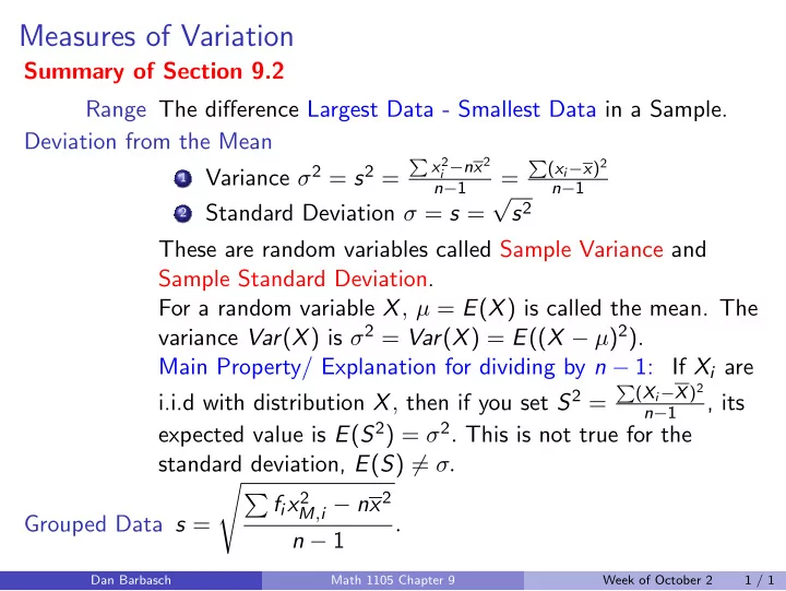
Summary of Section 9.2 Range The difference Largest Data - Smallest Data in a Sample. Deviation from the Mean

1 Variance σ2 = s2 =

x2

i −nx2

n−1

=

(xi−x)2 n−1

2 Standard Deviation σ = s =

√ s2 These are random variables called Sample Variance and Sample Standard Deviation. For a random variable X, µ = E(X) is called the mean. The variance Var(X) is σ2 = Var(X) = E((X − µ)2). Main Property/ Explanation for dividing by n − 1: If Xi are i.i.d with distribution X, then if you set S2 =

(Xi−X)2 n−1

, its expected value is E(S2) = σ2. This is not true for the standard deviation, E(S) = σ. Grouped Data s = fix2

M,i − nx2

n − 1 .

Dan Barbasch Math 1105 Chapter 9 Week of October 2 1 / 1

Examples I

Example (Range)

Data 15, −3, 4, 7, 18. The smallest is −3, the largest 18 so Range = 18 − (−3) = 21. Always a nonnegative number.

Example (Deviation from the Mean)

In the previous example, x = 15−3+4+7+18

5

= 8.2. So 15 − 8.2 = 6.8, −3 − 8.2 = −11.2, 4 − 8.2 = −3.8, 7 − 8.2 = −1.2, 18 − 8.2 = 9.8.

Example (Variance and Standard Deviation)

s2 = 6.82+11.22+3.82+1.22+9.82

4

= 152+32+42+72+182−5·8.22

4

s = √ s2.

Dan Barbasch Math 1105 Chapter 9 Week of October 2 2 / 1

Examples II

Example (Binomial Distribution)

P(X = 1) = p, P(X = 0) = 1 − p. Then µ = E(X) = p, and σ2 = E((X − p)2) = (1 − p)2p + (0 − p)2(1 − p) = p(1 − p). This is the same as E(X 2 − p2) = (1 − p2)p + (−p2)(1 − p) = (1 − p)p. Remark: Note that the formula for variance and standard deviation only holds for n > 2. Otherwise, for n = 1, you would be dividing by 0. For one random variable, the variance is defined as Var(X) = E((X − E(X))2). For X1, X2,, two independent random variables, Var(X1 + X2) = Var(X1) + Var(X2). Suppose X is a random variable. We can write a table X a1 a2 . . . an P(X) p1 p2 . . . pn

Dan Barbasch Math 1105 Chapter 9 Week of October 2 3 / 1

Examples III

For the expected value µ = E(X), you multiply the two terms in each column, and add

• i

ai × pn = a1p1 + · · · + anpn. In a spreadsheet program, the data would be in columns and you would add over the products from the rows. You use a command like sumproduct to perform the operation. If you have some other variable like (X − µ)2, you would use the values (ai − µ)2 and the same pi.

Dan Barbasch Math 1105 Chapter 9 Week of October 2 4 / 1

Examples IV

Example

X 2 3 −1 1 X 2 4 9 1 1 (X − µ)2 (2 − 1/4)2 (3 − 1/4)2 (−1 − 1/4)2 (1 − 1/4)2 P(X) 1/2 1/8 1/4 1/8 Computing the expected values is below. µ = E(X) = (2) × (1/2) + (3) × (1/8) + (−1) × (1/4) + (1) × (1/8) = 1/4. Var(X) =(2 − 1/4)2 · (1/2) + (3 − 1/4)2 · (1/8) + (−1 − 1/4)2 · (1/4)+ +(1 − 1/4)2 · (1/8) = 47/16.

Dan Barbasch Math 1105 Chapter 9 Week of October 2 5 / 1

Normal Distribution I

Definition

Data are said to be normally distributed if the rate at which the frequencies fall off is proportional to the distance of the score from the mean, and to the frequencies themselves. This definition requires Calculus. We don’t assume or do Calculus in this

• course. We will however learn how to work with this distribution.

It is very useful in that many phenomena can be modeled by this. We will see how the binomial distribution is related to the normal distribution later in the chapter. Suppose you have a random variable X, and you would like to know about its mean µ. So you perform many n independent trials, and draw a

• histogram. The larger the n, the closer the outcome will look like the

curve f (x) =

1 √ 2πσe− (x−µ)2

2σ2 . The pictures in the text show what it looks

• like. The resulting probability is called N(µ, σ2), normal with mean µ and

Dan Barbasch Math 1105 Chapter 9 Week of October 2 6 / 1

Normal Distribution II

variance σ2. There is a precise statement called the Central Limit Theorem which says that for large n, √n(Sn − µ) “looks” like a normal distribution N(0, σ2). it is used in practice to model large populations and “ errors”. There are many examples that can be approximated by normal

• distributions. Heights of people, and scores on tests are examples.

This is not a finite distribution. For a random variable that is normally distributed, we write N(µ, σ2), P(X ≤ a) = the area under the normal curve from − ∞ to a. This is tabulated for µ = 0 and σ = 1. The rest is computed by simple formulas involving arithmetic.

Dan Barbasch Math 1105 Chapter 9 Week of October 2 7 / 1

Height Example I

Example (from the practice prelim)

• 8. (14 points) Assume that the height in inches of American women

follows a normal distribution with mean mu = 64′′ (5’4”) and standard deviation σ = 3′′. (a) (3 points) How many standard deviations above or below the mean is a height of 73” (6’1”)? (b) (4 points) What fraction of women are taller than 73 inches? (c) (4 points) In a room with 30 women, what is the probability that at least one of them is taller than 73”? (d) (3 points) What assumptions did you make when answering part (c)? Are there circumstances under which those assumptions would not be justified?

Dan Barbasch Math 1105 Chapter 9 Week of October 2 8 / 1

Height Example II

Answer.

(a) same as before 3 standard deviations away. (b) P(X ≥ 73) = P(X − 64 ≥ 73 − 64 = 9 = 3σ) = P(X − µ σ ≥ 3) = =1 − P(X − µ σ ≤ 3) = 1 − 0.999 = 0.001. This is 1/1000. The random variable X has probability distribution N(64, 17). The probability P(X ≥ 73) comes from this normal distribution. To actually look it up in the tables, you rewrite it in terms of Z = X−64

3

which has probability distribution N(0, 1). This is the one in the tables. (c) P(at least 1/30 ≥ 73) =1 − P(30/30 ≤ 73) = 1 − P(X ≤ 73)30 = =1 − (0.998)30.

Dan Barbasch Math 1105 Chapter 9 Week of October 2 9 / 1

z−value

The principle is X normal N(µ, σ2) ⇐ ⇒ Z = X−µ

σ

normal N(0, 1). So P(X ≤ a) = P(Z ≤ a − µ σ ). z = a−µ

σ

is called the z−value. This is what you look up in the tables.

Dan Barbasch Math 1105 Chapter 9 Week of October 2 10 / 1

Example with Grades

Example

A professor (not this one!) of a course wants to give grades so that A top 8% F bottom 8% B next 20% below A D next 20% above the F C the rest The mean is µ = 67 and the standard deviation is σ = 17. Find the cutoffs.

Answer.

P(≤ A) = 0.92 z = 1.41 a = µ + zσ = 67 + 17 · 1.41 = 91 P(≤ B) = 0.72 z = 0.58 a = µ + zσ = 67 + 17 · 0.58 = 77 P(≤ C) = 0.28 z = −.59 a = µ + zσ = 67 + 17 · (−.59) = 57 P(≤ D) = 0.08 z = −1.39 a = µ + zσ = 67 + 17 · (−1.39) = 43 from the tables. In Excel or alike you can write norminv(0.92, 67, 17) ∼ = 91.

Dan Barbasch Math 1105 Chapter 9 Week of October 2 11 / 1

Approximate Binomial Distribution by the Normal Dstribution I

Theorem

Let B = X1 + · · · + Xn be the binomial Distribution, coming from adding up Xi = X i.i.d. with P(X = 1) = p, P(X = 0) = 1 − p. Then E(B) = np, Var(B) = np(1 − p). The normal approxinmation of the binomial distribution is P(B ≤ a) ≃ P(Z ≤ a − np

• np(1 − p)

). where Z has the normal distribution N(0, 1). In other words, the binomial distribution is approximately the normal distribution with the same mean and variance, N(np, np(1 − p).

Dan Barbasch Math 1105 Chapter 9 Week of October 2 12 / 1

Approximate Binomial Distribution by the Normal Dstribution II

Remember the notation N(µ, σ2) for the normal distribution. σ2 is the variance, its square root σ is the standard deviation.

Example

Approximate C(100, 50).

Dan Barbasch Math 1105 Chapter 9 Week of October 2 13 / 1

Approximate Binomial Distribution by the Normal Dstribution III

Answer.

Use the binomial distribution with p = 0.5 and n = 100. C(100, 50) · (0.5)100 ≃ P(49.5 < B < 50.5). The mean is 100 · 0.5 = 50. The standard deviation is √ 100 · 0.5 · 0.5 = 5. So C(100, 50) ≃2100 · P 49.5 − 50 5 ≤ Z ≤ 50.5 − 50 5

• =

=0.5398 − 0.4602 = 0.08. You have to box in 50 by two numbers: 49.5 < 50 < 50.5 is a reasonable choice.

Dan Barbasch Math 1105 Chapter 9 Week of October 2 14 / 1

Drug Effectiveness I

Example (Drug Effectiveness, Problem 24 in 9.4)

A new drug cures 80% of the patients to whom it is administered. It is given to 25 patients. Find the probabilities that among these patients, the following results occur.

• a. Exactly 20 are cured.
• b. All are cured.
• c. No one is cured.
• d. Twelve or fewer are cured.

Dan Barbasch Math 1105 Chapter 9 Week of October 2 15 / 1

Drug Effectiveness II

Answer.

a) C(25, 20)(0.8)20(0.2)5 b) C(25, 25)(0.8)25 c) C(25, 0)(0.2)25 d) Sum over C(25, k)(0.8)k(0.2)25−k for 0 ≤ k ≤ 12. Use the interval −0.5 ≤ B(24, 0.8) ≤ 12.5.5. The mean is 25 · 0.8 = 20. The standard deviation is √ 25 · 0.8 · 0.2 = 2 P

• Z ≤ 12.5 − 20

2

• − P
• Z ≤ −0.5 − 20

2

• =

= P (Z ≤ −7.5) − P(Z ≤ −20.5) You can also write P

• Z ≤ 12.5 − 20

2

• = P (Z ≤ −3.75) < 0.0002. This

is not in the tables. 12.5 is more than 4 standard deviations away from the mean.

Dan Barbasch Math 1105 Chapter 9 Week of October 2 16 / 1

Continuity Correction I

This is an example off the web from a statistics course (Yale). Note: Because the normal approximation is not accurate for small values

• f n, a good rule of thumb is to use the normal approximation only if

np > 10 and np(1 − p) > 10. Sometimes people use 5 instead of 10.

Example

Consider a population of voters in a given state. The true proportion of voters who favor candidate A is equal to 0.40. Given a sample of 200 voters, what is the probability that more than half of the voters support candidate A?

Dan Barbasch Math 1105 Chapter 9 Week of October 2 17 / 1

Continuity Correction II

Answer.

The count X of voters in the sample of 200 who support candidate A is distributed B(200, 0.4). The mean of the distribution is equal to 200 ∗ 0.4 = 80, and the variance is equal to 200 ∗ 0.4 ∗ 0.6 = 48. The standard deviation is the square root of the variance, 6.93. The probability that more than half of the voters in the sample support candidate A is equal to the probability that X is greater than 100, which is equal to 1 − P(X < 100). More than half means strictly more than half. To use the normal approximation to calculate this probability, we should first acknowledge that the normal distribution is continuous and apply the continuity correction. This means that the probability for a single discrete value, such as 100, is extended to the probability of the interval (99.5, 100.5). Because we are interested in the probability that X is less than or equal to 100, the normal approximation applies to the upper limit

• f the interval, 100.5. If we were interested in the probability that X is

strictly less than 100, then we would apply the normal approximation to the lower end of the interval, 99.5.

Dan Barbasch Math 1105 Chapter 9 Week of October 2 18 / 1

Answer.

So, applying the continuity correction and standardizing the variable X gives the following: 1−P(X≤100) = 1 − P(X < 100.5)≃1 − P(Z < (100.5 − 80)/6.93) = = 1 − P(Z < 20.5/6.93) = 1 − P(Z < 2.96) = 1 − (0.9985) = 0.0015. Since the value 100 is nearly three standard deviations away from the mean 80, the probability of observing a count this high is extremely small. In the first two, it is the Binomial distribution, after that it is the standard normal distribution. Note: About 68% of values drawn from a normal distribution are within

• ne standard deviation σ away from the mean; about 95% of the values lie

within two standard deviations; and about 99.7% are within three standard

• deviations. This fact is known as the 68 − 95 − 99.7 (empirical) rule, or

the 3-sigma rule.

Dan Barbasch Math 1105 Chapter 9 Week of October 2 19 / 1