Implication Strength of Classification Rules Gilbert Ritschard - PowerPoint PPT Presentation
ISMIS, Bari, September 27-29, 2006 Implication Strength of Classification Rules Gilbert Ritschard Djamel A. Zighed University of Geneva, Switzerland ERIC, University of Lyon 2, France Outline 1 Introduction 2 Trees and implication indexes
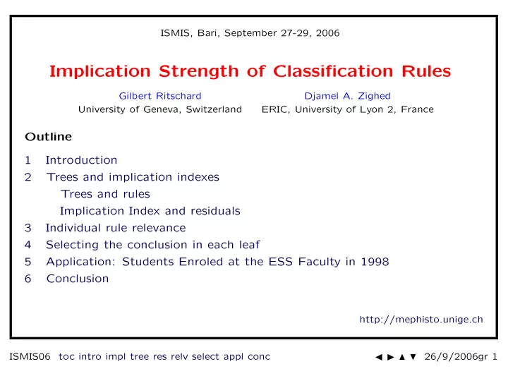
ISMIS, Bari, September 27-29, 2006 Implication Strength of Classification Rules Gilbert Ritschard Djamel A. Zighed University of Geneva, Switzerland ERIC, University of Lyon 2, France Outline 1 Introduction 2 Trees and implication indexes Trees and rules Implication Index and residuals 3 Individual rule relevance 4 Selecting the conclusion in each leaf 5 Application: Students Enroled at the ESS Faculty in 1998 6 Conclusion http://mephisto.unige.ch ISMIS06 toc intro impl tree res relv select appl conc ◭ ◮ � � 26/9/2006gr 1
1 Introduction • Implicative Statistics (IS) – Tool for data analysis (Gras, 1979) – Interestingness measure for association rules mining (Suzuki and Kodratoff, 1998; Gras et al., 2001) • IS useful for supervised classification? – YES, when the aim is characterizing typical profiles of outcomes Example 1: Physician interested in knowing typical profile of persons at risk for cancer, rather in predicting “cancer” or “not cancer” Example 2: Tax-collector interested in identifying groups where he has more chances to found fakers, rather in predicting “fraud” or “no fraud” – typical profile paradigm rather than classification paradigm ISMIS06 toc intro impl tree res relv select appl conc ◭ ◮ � � 26/9/2006gr 2
• Applying IS to decision rules • We focus on classification rules derived from decision trees. – Index of implication for classification rules ∗ Gras’s index as a standardized residual ∗ Alternative forms of residuals from modeling of contingency tables – Individual validation of classification rules – Optimal conclusion (alternative to the majority rule) ISMIS06 toc intro impl tree res relv select appl conc ◭ ◮ � � 26/9/2006gr 3
2 Trees and implication indexes 2.1 Trees and rules • Illustrative data set and example of induced tree • Classification rules and counter-examples (notations) ISMIS06 toc intro impl tree res relv select appl conc ◭ ◮ � � 26/9/2006gr 4
Illustrative data set (273 cases) Civil status Sex Activity sector Number of cases married male primary 50 married male secondary 40 married male tertiary 6 married female primary 0 married female secondary 14 married female tertiary 10 single male primary 5 single male secondary 5 single male tertiary 12 single female primary 50 single female secondary 30 single female tertiary 18 divorced/widowed male primary 5 divorced/widowed male secondary 8 divorced/widowed male tertiary 10 divorced/widowed female primary 6 divorced/widowed female secondary 2 divorced/widowed female tertiary 2 ISMIS06 toc intro impl tree res relv select appl conc ◭ ◮ � � 26/9/2006gr 5
� � � � � � � � � � � � Induced tree for civil status (married, single, divorced/widow) � � � � � � � � � � � � � � � � � � � � � � � � � � � � � � � � � � � � � � � � � � � � � � � � � � � � � � � � � � � � � � � � � � � � � � � � � � � � � � � � � � � � � � � � � � � � � � � � � � ISMIS06 toc intro impl tree res relv select appl conc ◭ ◮ � � 26/9/2006gr 6
Table associated to the induced tree Man Woman primary or secondary Etat civil secondary tertiary primary or tertiary total Married 90 6 0 24 120 Single 10 12 50 48 120 Divorced/widow 13 10 6 4 33 Total 113 28 56 76 273 Rules (majority class): R1. Man of primary or secondary sector ⇒ married ⇒ R2. Man of tertiary sector single R3. Woman of primary sector ⇒ single R4. Woman of secondary or tertiary sector ⇒ single ISMIS06 toc intro impl tree res relv select appl conc ◭ ◮ � � 26/9/2006gr 7
Counter-examples Gras’s Implication Index defined from counter-examples. Counter-example: verifies premise, but not conclusion (classification error) Notations: b conclusion of rule j (changes with j ) n b · total number of cases verifying b , n ¯ b · = n − n b · (changes with j ) n bj number of cases with premise j which verify conclusion b n ¯ number of counter-examples for rule j bj Hypothesis that distribution among b and ¯ H 0 b is independent of the condition (same as marginal distribution) Number of counter-examples under H 0 : bj ∼ Poisson ( n e N ¯ bj ) ¯ bj | H 0 ) = n e with E( N ¯ bj | H 0 ) = Var( N ¯ bj = n ¯ b · n · j /n . (!!! b changes with j ) ¯ ISMIS06 toc intro impl tree res relv select appl conc ◭ ◮ � � 26/9/2006gr 8
Observed counts n ¯ bj and n bj of counter-examples et examples predicted Man Woman class primary or secondary secondary tertiary primary or tertiary total cpred 0 (counter-example) 23 16 6 28 73 1 (example) 90 12 50 48 200 Total 113 28 56 76 273 Expected counts n e bj and n e bj of counter-examples et examples (Indep) ¯ predicted Man Woman class primary or secondary secondary tertiary primary or tertiary total cpred 0 (counter-example) 63.33 15.69 31.38 42.59 153 1 (example) 49.67 12.31 24.62 33.41 120 Total 113 28 56 76 273 ISMIS06 toc intro impl tree res relv select appl conc ◭ ◮ � � 26/9/2006gr 9
2.2 Implication Index and residuals bj − n e n ¯ ¯ bj Imp ( j ) = � n e ¯ bj Contribution to Chi-square measuring distance between observed and expected predicted Man Woman class primary or secondary secondary tertiary primary or tertiary cpred 0 (counter-example) -5.068 0.078 -4.531 -2.236 1 (example) 5.722 -0.088 5.116 2.525 bj ) 2 bj − n e bj ) 2 ( n ¯ ( n bj − n e � � ¯ χ 2 = + n e n e ¯ bj bj j j � �� � Imp 2 ( j ) ISMIS06 toc intro impl tree res relv select appl conc ◭ ◮ � � 26/9/2006gr 10
Alternative residuals (used in statistical modeling of contingency tables) standardized (=Imp ( j ) ) res s contribution to Pearson Chi-square res d deviance contribution to Likelihood-ratio Chi-square (Bishop et al., 1975, p 136) res a res s divided by its standard error adjusted (Haberman) (Agresti, 1990, p 224) res T F Freeman-Tukey variance stabilization (Bishop et al., 1975, p 137) Residual Rule 1 Rule 2 Rule 3 Rule 4 standardized ( = Imp ( j ) ) res s -5.068 0.078 -4.531 -2.236 deviance res d -6.826 0.788 -4.456 -4.847 Freeman-Tukey res F T -6.253 0.138 -6.154 -2.414 adjusted res a -9.985 0.124 -7.666 -3.970 n e bj is mere an estimation ⇒ variance of Imp ( j ) < 1 ¯ and Imp ( j ) tends to under-estimate the implication strength. Other residuals are closer to N (0 , 1) . ISMIS06 toc intro impl tree res relv select appl conc ◭ ◮ � � 26/9/2006gr 11
Degree of significance of the implication index p -value of implication index = p ( N ¯ bj ≤ n ¯ bj | H 0 ) . Prob. to get, by chances under H 0 , less counter-examples than observed Assuming fixed n b · and n · j , can be computed • with Poisson when n is small • normal approximation when n is large ( ≥ 5 ) For normal approximation: continuity correction (add 0.5 to observed counts) Difference may be as large as 2.6 points of percentage when n ¯ bj = 100 . ISMIS06 toc intro impl tree res relv select appl conc ◭ ◮ � � 26/9/2006gr 12
Poisson, normal and normal with correction distributions 1 0.9 0.8 0.7 0.6 Poisson 0.5 Normal corr Normal 0.4 0.3 0.2 0.1 0 10 15 20 25 30 ISMIS06 toc intro impl tree res relv select appl conc ◭ ◮ � � 26/9/2006gr 13
Details of Poisson, normal and normal with correction distributions 0.6 0.5 0.4 Poisson 0.3 Normal Normal corr 0.2 0.1 0 15 16 17 18 19 ISMIS06 toc intro impl tree res relv select appl conc ◭ ◮ � � 26/9/2006gr 14
Implication intensity The smaller the p -value, the greater the intensity ⇒ Intensity of implication = complement to 1 of p -value Prob. to get, by chances under H 0 , more counter-examples than observed Gras et al. (2004) define it in terms the normal approximation, without continuity correction We use bj + 0 . 5 − n e � n ¯ � ¯ bj Intens ( j ) = 1 − φ � n e ¯ bj ISMIS06 toc intro impl tree res relv select appl conc ◭ ◮ � � 26/9/2006gr 15
Variants of implication intensities (with continuity correction) Residual Rule 1 Rule 2 Rule 3 Rule 4 res s standardized 1.000 0.419 1.000 0.985 res d deviance 1.000 0.099 1.000 1.000 Freeman-Tukey res F T 1.000 0.350 1.000 0.988 adjusted res a 1.000 0.373 1.000 1.000 Intensity < 0 . 5 ⇔ more counter-examples than expected under H 0 . ⇒ Rule 2 irrelevant, since it makes worse than chance for predicting “single”. ISMIS06 toc intro impl tree res relv select appl conc ◭ ◮ � � 26/9/2006gr 16
3 Individual rule relevance In classification and especially with trees, the performance of the classifier is usually evaluated globally for the whole set of rules, by means for instance of the overall classification error in generalization. The implication intensity and its variants may be used for validating the individual relevance of the rules . In our example • R1, R3 et R4 are clearly relevant • R2 is not What shall we do with non relevant rules? (Remember that the set of rule conditions must define a partition of the data set) ISMIS06 toc intro impl tree res relv select appl conc ◭ ◮ � � 26/9/2006gr 17
Recommend
More recommend
Explore More Topics
Stay informed with curated content and fresh updates.









![Classification Image Classification Set of predefined categories [eg: table, apple, dog, giraffe]](https://c.sambuz.com/743996/classification-s.webp)
