Old News Old News Reminder for H4 CPSC 314 Computer Graphics - - PowerPoint PPT Presentation

SLIDE 1

University of British Columbia CPSC 314 Computer Graphics Jan-Apr 2007 Tamara Munzner http://www.ugrad.cs.ubc.ca/~cs314/Vjan2007

Curves Week 12, Wed Apr 4

2

Old News

• extra TA office hours in lab for hw/project

Q&A

• next week: Thu 4-6, Fri 10-2
• last week of classes:
• Mon 2-5, Tue 4-6, Wed 2-4, Thu 4-6, Fri 9-6
• final review Q&A session
• Mon Apr 16 10-12
• reminder: no lecture/labs Fri 4/6, Mon 4/9

3

Old News

• project 4 grading slots signup
• Wed Apr 18 10-12
• Wed Apr 18 4-6
• Fri Apr 20 10-1

4

Reminder for H4

• For any answer involving calculation,

although it's fine to show your work in analytical form, the final answer should be expressed as a number to two decimal places.

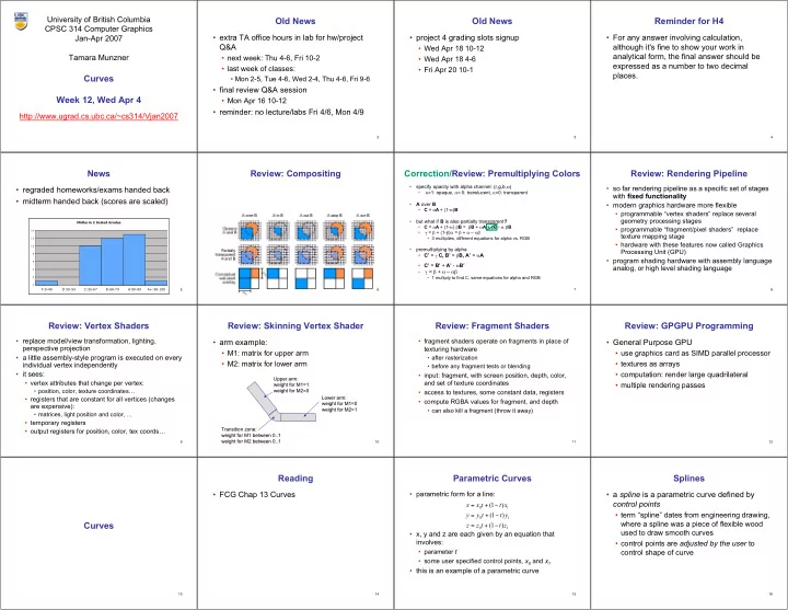
5

News

• regraded homeworks/exams handed back
• midterm handed back (scores are scaled)

Midterm 2 Scaled Grades 2 4 6 8 10 12 14 F:0-49 D:50-54 C:55-67 B:68-79 A:80-89 A+:90-100 6

Review: Compositing

7

Correction/Review: Premultiplying Colors

• specify opacity with alpha channel: (r,g,b,α)
• α=1: opaque, α=.5: translucent, α=0: transparent
• A over B
• C = αA + (1-α)B
• but what if B is also partially transparent?
• C = αA + (1-α) βB = βB + αA + βB - α βB
• γ = β + (1-β)α = β + α – αβ
• 3 multiplies, different equations for alpha vs. RGB
• premultiplying by alpha
• C’ = γ C, B’ = βB, A’ = αA
• C’ = B’ + A’ - αB’
• γ = β + α – αβ
• 1 multiply to find C, same equations for alpha and RGB

8

Review: Rendering Pipeline

• so far rendering pipeline as a specific set of stages

with fixed functionality

• modern graphics hardware more flexible
• programmable “vertex shaders” replace several

geometry processing stages

• programmable “fragment/pixel shaders” replace

texture mapping stage

• hardware with these features now called Graphics

Processing Unit (GPU)

• program shading hardware with assembly language

analog, or high level shading language

9

Review: Vertex Shaders

• replace model/view transformation, lighting,

perspective projection

• a little assembly-style program is executed on every

individual vertex independently

• it sees:
• vertex attributes that change per vertex:
• position, color, texture coordinates…
• registers that are constant for all vertices (changes

are expensive):

• matrices, light position and color, …
• temporary registers
• output registers for position, color, tex coords…

10

Review: Skinning Vertex Shader

• arm example:
• M1: matrix for upper arm
• M2: matrix for lower arm

Upper arm: Upper arm: weight for M1=1 weight for M1=1 weight for M2=0 weight for M2=0 Lower arm: Lower arm: weight for M1=0 weight for M1=0 weight for M2=1 weight for M2=1 Transition zone: Transition zone: weight for M1 between 0..1 weight for M1 between 0..1 weight for M2 between 0..1 weight for M2 between 0..1

11

Review: Fragment Shaders

• fragment shaders operate on fragments in place of

texturing hardware

• after rasterization
• before any fragment tests or blending
• input: fragment, with screen position, depth, color,

and set of texture coordinates

• access to textures, some constant data, registers
• compute RGBA values for fragment, and depth
• can also kill a fragment (throw it away)

12

Review: GPGPU Programming

• General Purpose GPU
• use graphics card as SIMD parallel processor
• textures as arrays
• computation: render large quadrilateral
• multiple rendering passes

13

Curves

14

Reading

• FCG Chap 13 Curves

15

Parametric Curves

• parametric form for a line:
• x, y and z are each given by an equation that

involves:

• parameter t
• some user specified control points, x0 and x1
• this is an example of a parametric curve

1 1 1

) 1 ( ) 1 ( ) 1 ( z t t z z y t t y y x t t x x − + = − + = − + =

16

Splines

• a spline is a parametric curve defined by

control points

• term “spline” dates from engineering drawing,

where a spline was a piece of flexible wood used to draw smooth curves

• control points are adjusted by the user to

control shape of curve

SLIDE 2 17

Splines - History

• draftsman used ‘ducks’ and

strips of wood (splines) to draw curves

• wood splines have second-
• rder continuity, pass

through the control points

a duck (weight) ducks trace out curve

18

Hermite Spline

• hermite spline is curve for which user

provides:

• endpoints of curve
• parametric derivatives of curve at endpoints
• parametric derivatives are dx/dt, dy/dt, dz/dt
• more derivatives would be required for higher
• rder curves

19

Basis Functions

• a point on a Hermite curve is obtained by multiplying each

control point by some function and summing

• functions are called basis functions
• 0.4
• 0.2

0.2 0.4 0.6 0.8 1 1.2 x1 x0 x'1 x'0 20

Sample Hermite Curves

21

Bézier Curves

• similar to Hermite, but more intuitive

definition of endpoint derivatives

• four control points, two of which are knots

22

Bézier Curves

• derivative values of Bezier curve at knots

dependent on adjacent points

23

Bézier Blending Functions

• look at blending functions
• family of polynomials called
• rder-3 Bernstein polynomials
• C(3, k) tk (1-t)3-k; 0<= k <= 3
• all positive in interval [0,1]
• sum is equal to 1

24

Bézier Blending Functions

• every point on curve is linear

combination of control points

• weights of combination are all

positive

• sum of weights is 1
• therefore, curve is a convex

combination of the control points

25

Bézier Curves

• curve will always remain within convex hull

(bounding region) defined by control points

26

Bézier Curves

• interpolate between first, last control points
• 1st point’s tangent along line joining 1st, 2nd pts
• 4th point’s tangent along line joining 3rd, 4th pts

27

Comparing Hermite and Bézier

0.2 0.4 0.6 0.8 1 1.2 B0 B1 B2 B3

• 0.4
• 0.2

0.2 0.4 0.6 0.8 1 1.2 x1 x0 x'1 x'0

Bézier Hermite

28

Rendering Bezier Curves: Simple

• evaluate curve at fixed set of parameter values, join

points with straight lines

• advantage: very simple
• disadvantages:
• expensive to evaluate the curve at many points
• no easy way of knowing how fine to sample points,

and maybe sampling rate must be different along curve

• no easy way to adapt: hard to measure deviation of

line segment from exact curve

29

Rendering Beziers: Subdivision

• a cubic Bezier curve can be broken into two

shorter cubic Bezier curves that exactly cover

• riginal curve
• suggests a rendering algorithm:
• keep breaking curve into sub-curves
• stop when control points of each sub-curve

are nearly collinear

• draw the control polygon: polygon formed by

control points

30

Sub-Dividing Bezier Curves

• step 1: find the midpoints of the lines joining

the original control vertices. call them M01, M12, M23

P0 P1 P2 P3 M01 M12 M23

31

Sub-Dividing Bezier Curves

• step 2: find the midpoints of the lines joining

M01, M12 and M12, M23. call them M012, M123

P0 P1 P2 P3 M01 M12 M23 M012 M123

32

Sub-Dividing Bezier Curves

• step 3: find the midpoint of the line joining

M012, M123. call it M0123

P0 P1 P2 P3 M01 M12 M23 M012 M123 M0123

SLIDE 3 33

Sub-Dividing Bezier Curves

• curve P0, M01, M012, M0123 exactly follows original

from t=0 to t=0.5

• curve M0123 , M123 , M23, P3 exactly follows
• riginal from t=0.5 to t=1

P0 P1 P2 P3 M01 M12 M23 M012 M123 M0123

34

Sub-Dividing Bezier Curves

P0 P1 P2 P3

• continue process to create smooth curve

35

de Casteljau’s Algorithm

• can find the point on a Bezier curve for any parameter

value t with similar algorithm

• for t=0.25, instead of taking midpoints take points 0.25 of

the way

P0 P1 P2 P3 M01 M12 M23 t=0.25

demo: www.saltire.com/applets/advanced_geometry/spline/spline.htm

36

Longer Curves

• a single cubic Bezier or Hermite curve can only capture a small class of

curves

• at most 2 inflection points
• ne solution is to raise the degree
• allows more control, at the expense of more control points and higher

degree polynomials

• control is not local, one control point influences entire curve
• better solution is to join pieces of cubic curve together into piecewise

cubic curves

• total curve can be broken into pieces, each of which is cubic
• local control: each control point only influences a limited part of the

curve

• interaction and design is much easier

37

Piecewise Bezier: Continuity Problems

demo: www.cs.princeton.edu/~min/cs426/jar/bezier.html

38

Continuity

• when two curves joined, typically want some

degree of continuity across knot boundary

• C0, “C-zero”, point-wise continuous, curves

share same point where they join

• C1, “C-one”, continuous derivatives
• C2, “C-two”, continuous second derivatives

39

Geometric Continuity

• derivative continuity is important for animation
• if object moves along curve with constant parametric

speed, should be no sudden jump at knots

• for other applications, tangent continuity suffices
• requires that the tangents point in the same direction
• referred to as G1 geometric continuity
• curves could be made C1 with a re-parameterization
• geometric version of C2 is G2, based on curves

having the same radius of curvature across the knot

40

Achieving Continuity

• Hermite curves
• user specifies derivatives, so C1 by sharing points and derivatives

across knot

• Bezier curves
• they interpolate endpoints, so C0 by sharing control pts
• introduce additional constraints to get C1
• parametric derivative is a constant multiple of vector joining first/last 2

control points

• so C1 achieved by setting P0,3=P1,0=J, and making P0,2 and J and P1,1

collinear, with J-P0,2=P1,1-J

• C2 comes from further constraints on P0,1 and P1,2
• leads to...

41

B-Spline Curve

• start with a sequence of control points
• select four from middle of sequence

(pi-2, pi-1, pi, pi+1)

• Bezier and Hermite goes between pi-2 and pi+1
• B-Spline doesn’t interpolate (touch) any of them but

approximates the going through pi-1 and pi

P0 P1 P3 P2 P4 P5 P6

42

B-Spline

• by far the most popular spline used
• C0, C1, and C2 continuous

demo: www.siggraph.org/education/materials/HyperGraph/modeling/splines/demoprog/curve.html 43

B-Spline

• locality of points