Likelihood functions Setting: Let Y 1 , ..., Y n be independent - - PowerPoint PPT Presentation

likelihood functions setting let y 1 y n be independent
SMART_READER_LITE
LIVE PREVIEW

Likelihood functions Setting: Let Y 1 , ..., Y n be independent - - PowerPoint PPT Presentation

Likelihood functions Setting: Let Y 1 , ..., Y n be independent random variables, with Y i having density (or probability) function f ( y i | ) , where is some unknown parameter. For example, in the Bernoulli distribution, all the Y i


slide-1
SLIDE 1

Likelihood functions

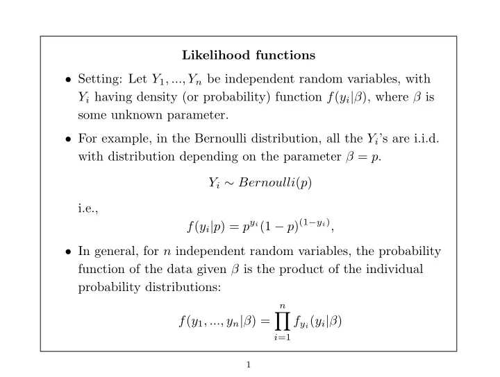
  • Setting: Let Y1, ..., Yn be independent random variables, with

Yi having density (or probability) function f(yi|β), where β is some unknown parameter.

  • For example, in the Bernoulli distribution, all the Yi’s are i.i.d.

with distribution depending on the parameter β = p. Yi ∼ Bernoulli(p) i.e., f(yi|p) = pyi(1 − p)(1−yi),

  • In general, for n independent random variables, the probability

function of the data given β is the product of the individual probability distributions: f(y1, ..., yn|β) =

n

  • i=1

fyi(yi|β)

1

slide-2
SLIDE 2
  • The Likelihood function of β given the data are equivalent

to the probability function of the data given β: L(β) = L(β|y1, ..., yn) =

n

  • i=1

fyi(yi|β).

  • Once you take the random sample of size n, the Yi’s are known,

but β is not – in fact, the only unknown in the likelihood is the parameter β.

  • Example: The Likelihood function of p for a sample of n

Bernoulli r.v.’s is: L(p) =

n

  • i=1

pyi(1 − p)(1−yi) = p

n

i=1 yi(1 − p)n−n i=1 yi

2

slide-3
SLIDE 3
  • Maximum Likelihood Estimator (MLE) of β -

the value, ˆ β, which maximizes the likelihood L(β) or the log-likelihood log L(β) as a function of β, given the observed Yi’s.

  • The value ˆ

β that maximizes L(β) also maximizes log L(β), since the latter is a monotone function of L(β).

  • It is usually easier to maximize log L(β), (why?)

so we focus on the log-likelihood.

  • Most of the estimates we will discuss in this class will be

MLE’s.

3

slide-4
SLIDE 4
  • For most distributions, the maximum is found by solving

∂ log L(β) ∂β = 0

  • Technically, we need to verify that we are at a maximum

(rather than a minimum) by seeing if the second derivative is negative at ˆ β, i.e., ∂2 log L(β) ∂β2

  • β= ˆ

β

< 0

  • The opposite of the second derivative, − ∂2 log L(β)

dβ2

, is called the “information”. This quantity plays an important part in likelihood theory.

4

slide-5
SLIDE 5

Example: Bernoulli data

  • The likelihood is

L(p) = n

i=1 pyi(1 − p)1−yi

= py(1 − p)n−y, where Y =

n

  • i−1

Yi = number of successes

5

slide-6
SLIDE 6
  • The log-likelihood is

log L(p) = y log p + (n − y) log(1 − p),

  • The first derivative is

∂ log L(p) ∂p = y p − n − y 1 − p = y − np p(1 − p) Setting this to 0 and solving for p, you get

  • p = y

n

6

slide-7
SLIDE 7
  • The second derivative of the log-likelihood is

∂2 log L(p) ∂p2 = −y p2 − (n − y) (1 − p)2

  • Evaluating at p =

p: ∂2 log L(p) ∂p2

  • p=

p

= − y (y/n)2 − (n − y) (1 − (y/n))2 = −n2 y − n2 (n − y) <

  • When 0 < y < n, the 2nd derivative at

p is negative, so p is the maximum.

  • When y = 0 or y = n, the estimate

p = 0 or p = 1 is said to be

  • n the ‘boundary’.

7

slide-8
SLIDE 8

Properties of MLE’s Any two likelihoods, L1(β) and L2(β), that are proportional, i.e., L2(β) = α L1(β) (where α is a constant that does not depend on β) yield the same maximum likelihood estimator

8

slide-9
SLIDE 9
  • Example: If we had started with the Binomial distribution of

Y = n

i=1 Yi rather than n independent Bernoulli r.v.’s, then

the likelihood would be: f(y) =   n y   py(1 − p)n−y,

  • For this distribution, the log-likelihood is

log L(p) = log   n y   + y log p + (n − y) log(1 − p),

9

slide-10
SLIDE 10
  • The first derivative of the binomial log-likelihood is

∂ log L(p) ∂p

=

∂ ∂p

 log   n y     + ∂[y log p+(n−y) log(1−p)]

∂p

= 0 + ∂[y log p+(n−y) log(1−p)]

∂p

=

∂[y log p+(n−y) log(1−p)] ∂p

This is exactly the same as the first derivative of the log-likelihood for n independent Bernoulli’s.

  • Therefore, we get the same MLE for independent Bernoulli

data and Binomial data (both are based on Y = n

i=1 Yi )

  • The likelihood, L2(p) of the Binomial data is proportional to

10

slide-11
SLIDE 11

the likelihood, L1(p) based on the original Bernoulli data, since L2(p) = αL1(p) where α =   n y  

11

slide-12
SLIDE 12

Asymptotic Properties of MLE’s

  • The exact distribution of the MLE can be very complicated, so

we often have to rely on large sample methods instead.

  • Using a Taylor series expansion and the Delta Method, the

following properties can be shown as n → ∞ : (1) ˆ β is asymptotically unbiased∗: E(ˆ β) → β (2) ˆ β is consistent: pr{|ˆ β − β| > ǫ} → 0, (3) ˆ β is asymptotically efficient (it achieves the minimum variance among all asymptotically unbiased estimators)

∗ - (Note that it may be biased in small samples) 12

slide-13
SLIDE 13
  • In addition, using the Central Limit Theorem, it can be shown

that MLE’s are asymptotically normally distributed, i.e, ˆ β

·

∼ N[β, V ar(ˆ β)], where V ar(ˆ β) is the inverse of the expected value of the information: V ar(ˆ β) = −

  • E

∂2 log L(β) ∂β2 −1 , (Note, however, that V ar(ˆ β) is itself a function of β. We will come back to examine this issue later)

13

slide-14
SLIDE 14

Example: Bernoulli data (continued)

  • From the above MLE theory, we know that, for large n,
  • p

·

∼ N[p, V ar( p)] where V ar( p) = −

  • E

d2 log L(p) dp2 −1 ,

  • Recall, the second derivative of the log-likelihood is

∂2 log L(p) ∂p2 = − y p2 − (n − y) (1 − p)2 so that the ’information’ equals −∂2 log L(p) ∂p2 = y p2 + (n − y) (1 − p)2

14

slide-15
SLIDE 15
  • The expected value of the information is

E

  • −∂2 log L(p)

∂p2

  • =

E(Y ) p2 + E(n − Y ) (1 − p)2 = np p2 + n(1 − p) (1 − p)2 = n p + n (1 − p) = n p(1 − p)

15

slide-16
SLIDE 16
  • To get the asymptotic variance, we now take the inverse:

V ar( p) =

  • n

p(1 − p) −1 = p(1 − p) n

  • This confirms what we already derived using the CLT:
  • p

·

∼ N

  • p, p(1 − p)

n

  • 16
slide-17
SLIDE 17

MLE’s of functions The MLE of a function is the function of the MLE, i.e., The MLE of g(β) is g(ˆ β) Variance of g(ˆ β): Two possible methods for calculating the variance are: (1) Apply the Delta Method to g(ˆ β) According to the Delta method the variance of the function g(ˆ β) is V ar[g(ˆ β)] = [g′(β)]2V ar(ˆ β) (2) Rewrite the likelihood in terms of θ = g(β), then take the second derivative of the corresponding log-likelihood with respect to θ.

17

slide-18
SLIDE 18

Example: Binomial data

  • The MLE of p is

p = Y

n . What is the MLE of logit(p)?

  • Using the above result, the MLE of logit(p) is logit( Y

n )

  • Calculating V ar(logit(

p)): – Method (1): already shown – Method (2): Let θ = logit(p) = log (p/(1 − p)) . After some algebra, you can show that p = eθ 1 + eθ

18

slide-19
SLIDE 19

Substitute eθ/(1 + eθ) for p in the likelihood: f(y) =   n y   py(1 − p)n−y =   n y  

1+eθ

y 1 −

eθ 1+eθ

n−y Then take 2nd derivatives of the log-likelihood with respect to θ to find the information, and compute the inverse.

19

slide-20
SLIDE 20

Confidence Intervals and Hypothesis Testing

  • I. Confidence Intervals
  • From MLE theory, we know that for large n,
  • p

·

∼ N

  • p, p(1 − p)

n

  • A 95% confidence interval for p can thus be constructed as:
  • p ± 1.96
  • p(1 − p)

n However, we do not know p in the variance.

20

slide-21
SLIDE 21
  • Since

p is a consistent estimate of p, we can replace p(1 − p) in the variance by

  • p(1 −

p), and still get 95% coverage (in large samples).

  • Therefore, a large sample confidence interval for p is:
  • p ± 1.96
  • p(1 −

p) n .

21

slide-22
SLIDE 22

Large Sample Confidence Interval for β

  • In general, suppose we want a 95% confidence interval for β.

For large n, we know that ˆ β

·

∼ N[β, V ar(ˆ β)], where V ar(ˆ β) is the inverse of the expected value of the information, and is a function of β.

  • If we knew β in V ar(ˆ

β), we could form an asymptotic 95% confidence interval for β with ˆ β ± 1.96

  • V ar(ˆ

β). (But.... if we knew β, we wouldn’t need a confidence interval in the first place!)

22

slide-23
SLIDE 23
  • Since we do not know β, we have to estimate V ar(ˆ

β) by replacing β with its consistent estimator ˆ β :

  • V ar(ˆ

β) = [V ar(ˆ β)]β= ˆ

β

  • Then the confidence interval

ˆ β ± 1.96

  • V ar(ˆ

β), will have coverage of 95% in large samples.

23

slide-24
SLIDE 24

Confidence Interval for a Function of β A large sample 95% confidence interval for g(β) is g(ˆ β) ± 1.96

  • V ar[g(ˆ

β)] where

  • V ar[g(ˆ

β)] = {V ar[g(ˆ β)]}β= ˆ

β 24

slide-25
SLIDE 25

Some motivation for this result:

  • Using the Delta method, we know that for large samples,

g(ˆ β)

·

∼ N{g(β), V ar[g(ˆ β)]}. where V ar[g(ˆ β)] = [g′(β)]2[V ar(ˆ β)]}, is a function of β.

  • Since ˆ

β is a consistent estimate of β for large samples, we can substitute ˆ β for β in our estimate of the variance, i.e., V ar(ˆ β).

25

slide-26
SLIDE 26

Example: 95% confidence interval for g(p) = logit(p):

  • From MLE theory and the Delta method, we know that

logit( p)

·

∼ N

  • logit(p),
  • 1

np(1 − p)

  • We can obtain a 95% confidence interval for logit(p) by

replacing p in the variance with p, logit( p) ± 1.96

  • 1

n p(1 − p),

26

slide-27
SLIDE 27
  • II. Hypothesis Testing
  • A. Wald Tests
  • Suppose we want to test H0 : β = β∗.
  • For example, for data that follows a Binomial distribution, we

may be interested in testing H0 : p = 0.5

  • Under the null hypothesis, the large sample distribution of

p is:

  • p

·

∼ N[0.5, 0.5(1 − 0.5)/n]

27

slide-28
SLIDE 28
  • To test the null, you can use

Z1 = ( p − 0.5)

  • p (1 −

p)/n ∼ N(0, 1), in which p in V ar( p) is estimated by replacing p by p

  • Alternatively, you can use

Z2 = ( p − 0.5)

  • 0.5 (1 − 0.5)/n

∼ N(0, 1), in which p in V ar(p) is determined by replacing p by p = 0.5 (its value under the null).

28

slide-29
SLIDE 29

Wald Tests, cont’d In general, the following Wald Test statistics can be used to test the null hypothesis H0 : β = β∗ Z1 =

ˆ β−β∗

  • V ar( ˆ

β) ·

∼ N(0, 1)

  • r

Z2 =

ˆ β−β∗

[V ar( ˆ β)]β=β∗ ·

∼ N(0, 1)

29

slide-30
SLIDE 30

Motivation for these test statistics:

  • Based on large sample properties of MLE’s:

ˆ β ∼ N{β∗, [V ar(ˆ β)]}

  • We already saw that for constructing confidence intervals, we

can replace β by its consistent estimator ˆ β in V ar(ˆ β). This motivates use of Z1.

  • Under the null hypothesis, an alternative is to rely on the

assumption that β = β∗, and replace β by β∗ in V ar(ˆ β). This motivates use of Z2.

  • Since the square of a N(0, 1) r.v. follows a χ2

1 distribution, we

can also use the test statistics Z2

1 or Z2 2. 30

slide-31
SLIDE 31
  • B. Likelihood Ratio Tests

In large samples, under the null hypothesis H0 : β = β∗, it can be shown that: 2 log

  • L(ˆ

β|HA) L(β∗|H0)

  • = 2[log L(ˆ

β|HA) − log L(β∗|H0)]

·

∼ χ2

1

where L(ˆ β|HA) is the likelihood after replacing β by its estimate, ˆ β, under the alternative (HA), and L(β∗|H0) is the likelihood after replacing β by its specified value, β∗, under the null (H0).

31

slide-32
SLIDE 32

Example: Binomial Data

  • Suppose we are interested in testing H0 : p = 0.5.

For Binomial data, recall that the log-likelihood equals log L(p) = log   n y   + y log p + (n − y) log(1 − p),

  • Under the alternative,

log L( p|HA) = log   n y   + y log p + (n − y) log(1 − p)

32

slide-33
SLIDE 33
  • Under the null,

log L(0.5|H0) = log   n y   + y log(0.5) + (n − y) log(1 − 0.5)

  • Then the likelihood ratio statistic is

2  log   n y   + y log p + (n − y) log(1 − p)   −2  log   n y   + y log(0.5) + (n − y) log(1 − 0.5)   = 2

  • y log
  • p

0.5

  • + (n − y) log
  • 1−

p 1−0.5

  • which is approximately χ2

1. 33

slide-34
SLIDE 34
  • Note, we would get the same likelihood ratio statistic if we had

also used the likelihood associated with n independent Bernoulli r.v.’s. The log-likelihood would not contain the term log   n y   but this term subtracts out in the likelihood ratio statistic, since it is not a function of p, and thus is the same under the null and alternative.

  • In other words, any two likelihoods that are proportional will

yield the same likelihood ratio statistic.

34

slide-35
SLIDE 35
  • C. Score Tests
  • The SCORE TEST statistic is based on the first derivative of

the log-likelihood evaluated under the null hypothesis.

  • The first derivative of the log-likelihood is often referred to as

the “score”, and is denoted by U(β) = ∂ log L(β) ∂β =

n

  • i=1

∂ log Li(β) ∂β where Li(β) is the likelihood from the i-th observation.

  • Since the score can also be written as a sum of independent
  • bservations, we can apply the Central Limit Theorem to show

that it is approximately normal. Using the CLT, we obtain: U(β∗)

·

∼ N(E[U(β∗)], V ar[U(β∗)])

35

slide-36
SLIDE 36

However, it turns out that E[U(β∗)] always equals 0. So the asymptotic distribution can be simplified to: U(β∗)

·

∼ N(0, V ar[U(β∗)])

  • In general, the score test statistic for testing H0 : β = β∗ is:

Z = U(β∗)

  • V ar[U(β∗)]

·

∼ N(0, 1)

36

slide-37
SLIDE 37

Example: Test for Binomial Data:

  • For Binomial data, we showed that the first derivative of the

log-likelihood with respect to p is ∂ log L(p) ∂p = y − np p(1 − p) =

n

  • i=1

yi − p p(1 − p)

37

slide-38
SLIDE 38
  • The score test statistic for H0 : p = p∗ is:

Z = U(p∗) − E[U(p∗)]

  • V ar[U(p∗)]

=

  • y−np∗

p∗(1−p∗)

  • − E
  • y−np∗

p∗(1−p∗)

  • V ar
  • y−np∗

p∗(1−p∗)

  • and Z

·

∼ N(0, 1).

38

slide-39
SLIDE 39
  • Next, we need to find the MEAN and VARIANCE of U(p)

under the null hypothesis Under the null p = p∗ E[U(p∗)] = E(Y − np∗) p∗(1 − p∗) = 0 and V ar[U(p∗)] =

V ar(Y −np∗) [p∗(1−p∗)]2

=

np∗(1−p∗) [p∗(1−p∗)]2

=

n p∗(1−p∗), 39

slide-40
SLIDE 40
  • Given this mean and variance, the score statistic is

Z =

  • y−np∗

p∗(1−p∗)

  • − E
  • y−np∗

p∗(1−p∗)

  • V ar
  • y−np∗

p∗(1−p∗)

  • =
  • y−np∗

p∗(1−p∗)

  • − 0
  • n

p∗(1−p∗)

  • =

y − np∗

  • n[p∗(1 − p∗)]

and Z

·

∼ N(0, 1).

40

slide-41
SLIDE 41
  • Suppose we are interested in testing H0 : p = 0.5 then,

Z =

u(0.5)

V ar[u(0.5)]

=

y−0.5n

n[0.5(1−0.5)]

=

[y−0.5n]/n [√ n[0.5(1−0.5)]]/n

=

  • p−0.5

0.5(1−0.5)/n

and Z

·

∼ N(0, 1).

41

slide-42
SLIDE 42

Notes on Score Tests vs Wald and LR Tests:

  • Note that the SCORE statistic and the Wald statistic Z2 (with

the variance calculated under the null) are identical for this particular example. This is not usually the case.

  • In more complicated problems, Score test statistics are often

the easiest to calculate since you only need β∗ under the null, whereas the Likelihood Ratio and Wald statistics both use estimates of β under the alternative. Thus, Score statistics are

  • ften popular for their simplicity.
  • In large samples, all three test statistics (Score, Wald,

Likelihood ratio) are numerically almost identical if the null hypothesis is true. However, if the alternative is true, the power of the three may be different.

42