Likelihood Functions The likelihood function answers the question: - - PowerPoint PPT Presentation

Likelihood Functions

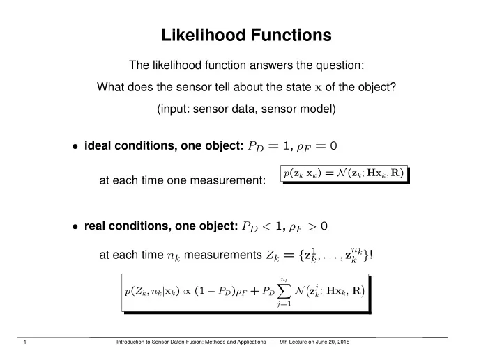
The likelihood function answers the question: What does the sensor tell about the state x of the object? (input: sensor data, sensor model)

• ideal conditions, one object: PD = 1, ρF = 0

at each time one measurement:

p(zk|xk) = N(zk; Hxk, R)

• real conditions, one object: PD < 1, ρF > 0

at each time nk measurements Zk = {z1

k, . . . , znk k }! p(Zk, nk|xk) / (1 PD)ρF + PD

nk

X

j=1

Nzj

k; Hxk, R

1 Introduction to Sensor Daten Fusion: Methods and Applications — 9th Lecture on June 20, 2018

Bayes Filtering for: PD < 1, ρF > 0, well-separated objects

state xk, current data Zk = {zj

k}mk j=1,

accumulated data Zk = {Zk, Zk1}

interpretation hypotheses Ek for Zk

• bject not detected, 1 PD

zk 2 Zk from object, PD

• mk + 1 interpretations

interpretation histories Hk for Zk

• tree structure: Hk = (EHk, Hk1) 2 Hk
• current: EHk, prehistories: Hki

p

• xk| Zk

=

X

Hk

p

• xk, Hk| Zk

=

X

Hk

p

• Hk| Zk

| {z }

weight!

pxk| Hk, Zk

| {z }

given Hk: unique

‘mixture’ density

2 Introduction to Sensor Daten Fusion: Methods and Applications — 9th Lecture on June 20, 2018

Closer look: PD < 1, ρF > 0, well-separated targets

filtering (at time tk1): p(xk1|Zk1) =

X

Hk1

pHk1 N

• xk1; xHk1, PHk1
• prediction (for time tk):

p(xk|Zk1) =

Z

dxk1 p(xk|xk1) p(xk1|Zk1) (MARKOV model) =

X

Hk1

pHk1 N

• xk; FxHk1, FPHk1F> + D
• measurement likelihood:

p(Zk, mk|xk) =

mk

X

j=0

p(Zk|Ej

k, xk, mk) P(Ej k|xk, mk)

(Ej

k: interpretations)

/ (1 PD) ρF + PD

mk

X

j=1

N

• zj

k; Hxk, R

• (H, R, PD, ρF)

filtering (at time tk): p(xk|Zk) / p(Zk, mk|xk) p(xk|Zk1) (BAYES’ rule) =

X

Hk

pHk N

• xk; xHk, PHk
• (Exploit product formula)

Sensor Data Fusion - Methods and Applications, 9th Lecture on June 20, 2018

Exercise: Show that p(xk|Zk) is given by Kalman updates and weights pj

Hk.

p(xk|Zk) =

mk

X

j=0

X

Hk1

pj

Hk1 N

⇣

xk1; xj

Hk1, Pj Hk1

⌘

pj

Hk1

= pj⇤

Hk1

P

j pj⇤ Hk1

pj⇤

Hk1

= pHk1

8 > > > > < > > > > :

(1 PD) ρF

j=0 PD

r

|2πSj

Hk1|

e

1

2νj> HkSj1 Hk1νj Hk

j6=0

Insert mixtures and exploit product formula in the numerator and denominator!

Sensor Data Fusion - Methods and Applications, 9th Lecture on June 20, 2018

Problem: Growing Memory Disaster:

m data, N hypotheses ! Nm+1 continuations

radical solution: mono-hypothesis approximation

Sensor Data Fusion - Methods and Applications, 9th Lecture on June 20, 2018

Problem: Growing Memory Disaster:

m data, N hypotheses ! Nm+1 continuations

radical solution: mono-hypothesis approximation

• gating: Exclude competing data with ||νi

k|k1|| > λ!

! KALMAN filter (KF) + very simple, λ too small: loss of target measurement

Sensor Data Fusion - Methods and Applications, 9th Lecture on June 20, 2018

Problem: Growing Memory Disaster:

m data, N hypotheses ! Nm+1 continuations

radical solution: mono-hypothesis approximation

• gating: Exclude competing data with ||νi

k|k1|| > λ!

! KALMAN filter (KF) + very simple, λ too small: loss of target measurement

• Force a unique interpretation in case of a conflict!

look for smallest statistical distance: mini ||νi

k|k1||

! Nearest-Neighbor filter (NN)

Sensor Data Fusion - Methods and Applications, 9th Lecture on June 20, 2018

Problem: Growing Memory Disaster:

m data, N hypotheses ! Nm+1 continuations

radical solution: mono-hypothesis approximation

• gating: Exclude competing data with ||νi

k|k1|| > λ!

! KALMAN filter (KF) + very simple, λ too small: loss of target measurement

• Force a unique interpretation in case of a conflict!

look for smallest statistical distance: mini ||νi

k|k1||

! Nearest-Neighbor filter (NN) + one hypothesis, hard decision, not adaptive

• global combining: Merge all hypotheses!

! PDAF, JPDAF filter + all data, + adaptive, reduced applicability

Sensor Data Fusion - Methods and Applications, 9th Lecture on June 20, 2018

PDAF Filter: formally analog to Kalman Filter

Filtering (scan k1): p(xk1|Zk1) = N(xk1; xk1|k1, Pk1|k1) (! initiation) prediction (scan k): p(xk|Zk1) ⇡ N(xk; xk|k1, Pk|k1) (like Kalman) Filtering (scan k): p(xk|Zk) ⇡

mk

X

j=0

pj

k N(xk; xj k|k, Pj k|k) ⇡ N(xk; xk|k, Pk|k)

νk

=

Pmk

j=0 pj k νj k ,

νj

k

= zj

k Hxk|k1

combined innovation

Wk

= Pk|k1H>S1

k ,

Sk

= HPk|k1H> + Rk Kalman gain matrix pj

k

= pi⇤

k / P j pj⇤ k ,

pj⇤

k

=

(

(1 PD) ρF

PD

p

|2πSHk| e 1

2ν> HkSHkνHk

weighting factors

xk = xk|k1 + Wk νk

(Filtering Update: Kalman)

Pk = Pk|k1 (1p0

k) WkSW> k

(Kalman part) + Wk

n Pmk

j=0 pj k νj kνj> k

νkνk>o

W>

k

(Spread of Innovations)

9 Introduction to Sensor Daten Fusion: Methods and Applications — 9th Lecture on June 20, 2018

The qualitative shape of p(xk|Zk) is often much simpler than its correct representation: a few pronounced modes

adaptive solution: nearly optimal approximation

Sensor Data Fusion - Methods and Applications, 9th Lecture on June 20, 2018

The qualitative shape of p(xk|Zk) is often much simpler than its correct representation: a few pronounced modes

adaptive solution: nearly optimal approximation

• individual gating: Exclude irrelevant data!

before continuing existing track hypotheses Hk1

! limiting case: KALMAN filter (KF)

Sensor Data Fusion - Methods and Applications, 9th Lecture on June 20, 2018

The qualitative shape of p(xk|Zk) is often much simpler than its correct representation: a few pronounced modes

adaptive solution: nearly optimal approximation

• individual gating: Exclude irrelevant data!

before continuing existing track hypotheses Hk1

! limiting case: KALMAN filter (KF)

• pruning: Kill hypotheses of very small weight!

after calculating the weights pHk, before filtering

! limiting case: Nearest Neighbor filter (NN)

Sensor Data Fusion - Methods and Applications, 9th Lecture on June 20, 2018

The qualitative shape of p(xk|Zk) is often much simpler than its correct representation: a few pronounced modes

adaptive solution: nearly optimal approximation

• individual gating: Exclude irrelevant data!

before continuing existing track hypotheses Hk1

! limiting case: KALMAN filter (KF)

• pruning: Kill hypotheses of very small weight!

after calculating the weights pHk, before filtering

! limiting case: Nearest Neighbor filter (NN)

• local combining: Merge similar hypotheses!

after the complete calculation of the pdfs

! limiting case: PDAF (global combining)

Sensor Data Fusion - Methods and Applications, 9th Lecture on June 20, 2018

Successive Local Combining

Partial sums of similar densities ! moment matching:

X

Hk2Hk⇤

pHk N(xk; xHk, PHk) ⇡ pH⇤

k N(xk; xH⇤ k, PH⇤ k)

Hk⇤ ⇢ Hk ! H⇤

k: effective hypothesis

Sensor Data Fusion - Methods and Applications, 9th Lecture on June 20, 2018

Successive Local Combining

Partial sums of similar densities ! moment matching:

X

Hk2Hk⇤

pHk N(xk; xHk, PHk) ⇡ pH⇤

k N(xk; xH⇤ k, PH⇤ k)

Hk⇤ ⇢ Hk ! H⇤

k: effective hypothesis

similarity: d(H1, H2) < µ mit (z.B.): d(H1, H2) = (xH1 xH2)>(PH1 + PH2)1(xH1 xH2) Start: Hypothesis of highest weight H1 ! search similar hypothesis (pH &) ! merge: (H1, H) H⇤

1 ! continue search (pH &) . . .

! restart: hypothesis with next to highest weight H2 ! . . .

Sensor Data Fusion - Methods and Applications, 9th Lecture on June 20, 2018

Successive Local Combining

Partial sums of similar densities ! moment matching:

X

Hk2Hk⇤

pHk N(xk; xHk, PHk) ⇡ pH⇤

k N(xk; xH⇤ k, PH⇤ k)

Hk⇤ ⇢ Hk ! H⇤

k: effective hypothesis

similarity: d(H1, H2) < µ mit (z.B.): d(H1, H2) = (xH1 xH2)>(PH1 + PH2)1(xH1 xH2) Start: Hypothesis of highest weight H1 ! search similar hypothesis (pH &) ! merge: (H1, H) H⇤

1 ! continue search (pH &) . . .

! restart: hypothesis with next to highest weight H2 ! . . .

• In many cases: good approximations ! quasi-optimality
• PDAF, JPDAF: Hk⇤ = Hk ! limited applicability
• robustness ! detail mostly irrelevant

Sensor Data Fusion - Methods and Applications, 9th Lecture on June 20, 2018

Retrodiction for GAUSSian Mixtures

wanted: p(xl|Zk) p(xl+1|Zk) for l < k p(xl|Zk) =

X

Hk

p(xl, Hk|Zk) =

X

Hk

p(xl|Hk, Zk)

| {z }

no ambiguities!

p(Hk|Zk)

| {z }

filtering!

Calculation of p(xl|Hk, Zk) as in case of PD = 1, ρF = 0! p(xl|Hk, Zk) = N

⇣

xl; xHk(l|k), PHk(l|k)

⌘

with parameters given by RAUCH-TUNG-STRIEBEL formulae:

xHk(l|k) = xHk(l|l) + WHk(l|k) (xHk(l+1|k) xHk(l+1|l)) PHk(l|k) = PHk(l|l) + WHk(l|k) (PHk(l+1|k) PHk(l+1|l)) WHk(l|k)>

gain matrix:

WHk(l|k) = PHk(l|l)F>

l+1|lPHk(l+1|l)1

Sensor Data Fusion - Methods and Applications, 9th Lecture on June 20, 2018

Retrodiction of Hypotheses’ Weights

Consider approximation: neglect RTS step!

p(xl|Hk, Zk) = N

• xl; xHk(l|k), PHk(l|k)
• ⇡ N
• xl; xHk(l|l), PHk(l|l)
• p(xl|Hk, Zk) ⇡

X

Hl

p⇤

Hl N

• xl; xHk(l|l), PHk(l|l)
• with recursively defined weights:

p⇤

Hk = pHk,

p⇤

Hl = P p⇤ Hl+1

summation over all histories Hl+1 with equal pre-histories!

• Strong sons strengthen weak fathers.
• Weak sons weaken even strong fathers.
• If all sons die, also the father must die.

Sensor Data Fusion - Methods and Applications, 9th Lecture on June 20, 2018

Track Extraction: Initiation of the PDF Iteration

extraction of target tracks: detection on a higher level of abstraction start: data sets Zk = {zj

k}mk j=1

(sensor performance: PD, ρF, R) goal: Detect a target trajectory in a time series: Zk = {Zi}k

i=1!

at first simplifying assumptions:

• The targets in the sensors’ field of view (FoV) are well-separated.
• The sensor data in the FoV in scan i are produced simultaneously.

Sensor Data Fusion - Methods and Applications, 9th Lecture on June 20, 2018

Track Extraction: Initiation of the PDF Iteration

extraction of target tracks: detection on a higher level of abstraction start: data sets Zk = {zj

k}mk j=1

(sensor performance: PD, ρF, R) goal: Detect a target trajectory in a time series: Zk = {Zi}k

i=1!

at first simplifying assumptions:

• The targets in the sensors’ field of view (FoV) are well-separated.
• The sensor data in the FoV in scan i are produced simultaneously.

decision between two competing hypotheses: h1: Besides false returns Zk contains also target measurements. h0: There is no target existing in the FoV; all data in Zk are false. statistical decision errors: P1 = Prob(accept h1|h1) analogous to the sensors’ PD P0 = Prob(accept h1|h0) analogous to the sensors’ PF

Sensor Data Fusion - Methods and Applications, 9th Lecture on June 20, 2018

Practical Approach: Sequential Likelihood Ratio Test

Goal: Decide as fast as possible for given decision errors P0, P1! Consider the ratio of the conditional probabilities p(h1|Zk), p(h0|Zk) and the likelihood ratio LR(k) = p(Zk|h1)/p(Zk|h0) as an intuitive decision function: p(h1|Zk) p(h0|Zk) = p(Zk|h1) p(Zk|h0) p(h1) p(h0) a priori: p(h1) = p(h0)

Sensor Data Fusion - Methods and Applications, 9th Lecture on June 20, 2018

Practical Approach: Sequential Likelihood Ratio Test

Goal: Decide as fast as possible for given decision errors P0, P1! Consider the ratio of the conditional probabilities p(h1|Zk), p(h0|Zk) and the likelihood ratio LR(k) = p(Zk|h1)/p(Zk|h0) as an intuitive decision function: p(h1|Zk) p(h0|Zk) = p(Zk|h1) p(Zk|h0) p(h1) p(h0) a priori: p(h1) = p(h0) Starting from a time window with length k = 1, calculate the test function LR(k) successively and compare it with two thresholds A, B: If LR(k) < A, accept hypothesis h0 (i.e. no target is existing)! If LR(k) > B, accept hypothesis h1 (i.e. target exists in FoV)! If A < LR(k) < B, wait for new data Zk+1, repeat with LR(k + 1)!

Sensor Data Fusion - Methods and Applications, 9th Lecture on June 20, 2018

Sequential LR Test: Some Useful Properties

• 1. Thresholds and decision errors are approximately related to each other by:

A ⇡ 1 P1 1 P0 and B ⇡ P1 P0

• 2. The actual decision length (number of scans required) is a random variable.
• 3. On average, the test has a minimal decision length for given errors P0, P1.
• 4. The quantity P0 (P1) affects the mean decision length given h1 (h0) holds.
• 5. Choose the probability P1 close to 1 for actually detecting real target tracks.
• 6. P0 should be small for not overloading the tracking system with false tracks.

23 Introduction to Sensor Daten Fusion: Methods and Applications — 9th Lecture on June 20, 2018

Iterative Calculation of the Likelihood Ratio

LR(k) = p(Zk|h1) p(Zk|h0) =

R

dxk p(Zk, mk, xk, Zk1|h1) p(Zk, mk, Zk1, h0)

Sensor Data Fusion - Methods and Applications, 9th Lecture on June 20, 2018

Iterative Calculation of the Likelihood Ratio

LR(k) = p(Zk|h1) p(Zk|h0) =

R

dxk p(Zk, mk, xk, Zk1|h1) p(Zk, mk, Zk1, h0) =

R

dxk p(Zk, mk|xk) p(xk|Zk1, h1) p(Zk1|h1) |FoV|mk pF(mk) p(Zk1|h0)

Sensor Data Fusion - Methods and Applications, 9th Lecture on June 20, 2018

Iterative Calculation of the Likelihood Ratio

LR(k) = p(Zk|h1) p(Zk|h0) =

R

dxk p(Zk, mk, xk, Zk1|h1) p(Zk, mk, Zk1, h0) =

R

dxk p(Zk, mk|xk) p(xk|Zk1, h1) p(Zk1|h1) |FoV|mk pF(mk) p(Zk1|h0) =

R

dxk p(Zk, mk|xk, h1) p(xk|Zk1, h1) |FoV|mk pF(mk) LR(k 1)

basic idea: iterative calculation!

Sensor Data Fusion - Methods and Applications, 9th Lecture on June 20, 2018

Iterative Calculation of the Likelihood Ratio

LR(k) = p(Zk|h1) p(Zk|h0) =

R

dxk p(Zk, mk, xk, Zk1|h1) p(Zk, mk, Zk1, h0) =

R

dxk p(Zk, mk|xk) p(xk|Zk1, h1) p(Zk1|h1) |FoV|mk pF(mk) p(Zk1|h0) =

R

dxk p(Zk, mk|xk, h1) p(xk|Zk1, h1) |FoV|mk pF(mk) LR(k 1)

basic idea: iterative calculation!

Let Hk = {Ek, Hk1} be an interpretation history of the time series Zk = {Zk, Zk1}. Ek = E0

k:

target was not detected, Ek = Ej

k: zj k 2 Zk is a target measurement.

p(xk|Zk1, h1) =

X

Hk1

p(xk|Hk1Zk1, h1) p(Hk1|Zk1, h1) The standard MHT prediction! p(Zk, mk|xk, h1, h1) =

X

Ek

p(Zk, Ek|xk, h1) The standard MHT likelihood function! The calculation of the likelihood ratio is just a by-product of Bayesian MHT tracking.

Sensor Data Fusion - Methods and Applications, 9th Lecture on June 20, 2018

Iteration Formula for LR(k) = p(Zk|h1)/p(Zk|h0)

initiation: k = 0,

j0 = 0,

λj0 = 1 recursion: LR(k + 1) =

X

jk+1

λjk+1 =

mk+1

X

jk+1=0

X

jk

λjk+1jk λjk

with:

λjk+1jk =

(

1 PD for jk+1 = 0

PD ρF N(νjk+1jk, Sjk+1jk)

for jk+1 6= 0 convenient notation: with jk = (jk, . . . , j1) let

X

jk

λjk =

mk

X

jk=0

· · ·

m1

X

j1=0

λjk...j1

Sensor Data Fusion - Methods and Applications, 9th Lecture on June 20, 2018

Iteration Formula for LR(k) = p(Zk|h1)/p(Zk|h0)

initiation: k = 0,

j0 = 0,

λj0 = 1 recursion: LR(k + 1) =

X

jk+1

λjk+1 =

mk+1

X

jk+1=0

X

jk

λjk+1jk λjk

with:

λjk+1jk =

(

1 PD for jk+1 = 0

PD ρF N(νjk+1jk, Sjk+1jk)

for jk+1 6= 0 innovation:

νjk+1jk = zjk+1 Hjk+1xjk+1|k

• innov. cov.:

Sjk+1jk = Hjk+1Pjk+1|kH>

jk+1 + Rjk+1

state update:

xjk+1|k = Fjk+1xjk xjk = xjk|k1 + Wjkjk1νjk,jk1

covariances:

Pjk+1|k = Fjk+1PjkF>

jk+1 + Djk+1

Pjk = Pjk|k1 Wjkjk1Sjkjk1W>

jkjk1

Sensor Data Fusion - Methods and Applications, 9th Lecture on June 20, 2018

Iteration Formula for LR(k) = p(Zk|h1)/p(Zk|h0)

initiation: k = 0,

j0 = 0,

λj0 = 1 recursion: LR(k + 1) =

X

jk+1

λjk+1 =

mk+1

X

jk+1=0

X

jk

λjk+1jk λjk

with:

λjk+1jk =

(

1 PD for jk+1 = 0

PD ρF N(νjk+1jk, Sjk+1jk)

for jk+1 6= 0 innovation:

νjk+1jk = zjk+1 Hjk+1xjk+1|k

• innov. cov.:

Sjk+1jk = Hjk+1Pjk+1|kH>

jk+1 + Rjk+1

state update:

xjk+1|k = Fjk+1xjk xjk = xjk|k1 + Wjkjk1νjk,jk1

covariances:

Pjk+1|k = Fjk+1PjkF>

jk+1 + Djk+1

Pjk = Pjk|k1 Wjkjk1Sjkjk1W>

jkjk1

Exercise 9.1 Show that this recursion formulae for calculating the decision function is true.

Sensor Data Fusion - Methods and Applications, 9th Lecture on June 20, 2018

Sequential Track Extraction: Discussion

• LR(k) is given by a growing number of summands, each related to a parti-

cular interpretation history. The tuple {λjk, xjk, Pjk} is called a sub-track.

Sensor Data Fusion - Methods and Applications, 9th Lecture on June 20, 2018

Sequential Track Extraction: Discussion

• LR(k) is given by a growing number of summands, each related to a parti-

cular interpretation history. The tuple {λjk, xjk, Pjk} is called a sub-track.

• For mitigating growing memory problems all approximations discussed for

track maintenance can be used if they do not significantly affect LR(k): – individual gating: Exclude data not likely to be associated. – pruning: Kill sub-tacks contributing marginally to the test function. – local combining: Merge similar sub tracks: {λi, xi, Pi}i ! {λ, x, P} with: λ = P

i λi,

x = 1

λ

P

i λixi,

P = 1

λ

P

i λi[Pi + (xi x)(. . .)>].

Sensor Data Fusion - Methods and Applications, 9th Lecture on June 20, 2018

Sequential Track Extraction: Discussion

• LR(k) is given by a growing number of summands, each related to a parti-

cular interpretation history. The tuple {λjk, xjk, Pjk} is called a sub-track.

• For mitigating growing memory problems all approximations discussed for

track maintenance can be used if they do not significantly affect LR(k): – individual gating: Exclude data not likely to be associated. – pruning: Kill sub-tacks contributing marginally to the test function. – local combining: Merge similar sub tracks: {λi, xi, Pi}i ! {λ, x, P} with: λ = P

i λi,

x = 1

λ

P

i λixi,

P = 1

λ

P

i λi[Pi + (xi x)(. . .)>].

• The LR test ends with a decision in favor of or against the hypotheses: h0

(no target) or h1 (target existing). Intuitive interpretation of the thresholds!

Sensor Data Fusion - Methods and Applications, 9th Lecture on June 20, 2018

track extraction at tk: Decide in favor of h1! initiation of pdf iteration (track maintenance):

Normalize coefficients λjk: pjk = λjk

P jk λjk

! (λjk, xjk, Pjk) ! p(xk|Zk) =

X jk

pjk N

⇣

xk; xjk, Pjk

⌘

Continue track extraction with the remaining sensor data!

sequential LR test for track monitoring:

After deciding in favor of h1 reset LR(0) = 1! Calculate LR(k) from p(xk|Zk)! track confirmation: LR(k) > P1

P0: reset LR(0) = 1!

track deletion: LR(k) < 1P1

1P0; ev. track re-initiation

Sensor Data Fusion - Methods and Applications, 9th Lecture on June 20, 2018

DEMONSTRATION (simulated)

Sensor Data Fusion - Methods and Applications, 9th Lecture on June 20, 2018

DEMONSTRATION (simulated)

Exercise 9.2 (voluntary) Simulate a detection process with a given PD, target measurements with a given R, a detection process with a given PD and realize the track extraction procedure.

Sensor Data Fusion - Methods and Applications, 9th Lecture on June 20, 2018

ABRAHAM WALD (1902-1950) Austro-Hungarian mathematician who contributed to decision theory, geometry, and econometrics; founded the theory of economic equilibria in Oskar Morgenstern’s institut in Vienna: “Berechnung der Ausschaltung von Saisonschwankungen” (Springer Verlag, 1936) the basis of Game Theory: Morgenstern, John von Neumann, John Forbes Nash (1994: Nobel price with Reinhard Selten, Bonn University) ! sensor management! Founder of statistical sequential analysis in WW II. 1950 plenary talk at the International Congress of Mathematicians ICM, Cambridge (Mass.): “Basic ideas of a general theory of statistical decision rules” (1900: Hilbert’s 23 Problems). Student and friend: Jacob Wolfowitz (statistician, information theory), classical text book: “Coding Theorems of Information Theory” (1978). Posthumous attack by Ronald Fisher: “an incompetent book on statistics”, passionately defended by Jerzy Neyman as imminent a statistician as Fisher.

Sensor Data Fusion - Methods and Applications, 9th Lecture on June 20, 2018