Curve Fitting Re-visited, Bishop1.2.5 Maximum Likelihood Bishop - PowerPoint PPT Presentation

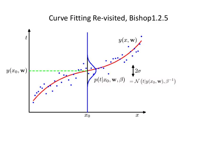
Curve Fitting Re-visited, Bishop1.2.5

Maximum Likelihood Bishop 1.2.5 Model • Likelihood • differentiation •

Maximum Likelihood N � N � t n | y ( x n , w ) , β − 1 � p ( t | x , w , β ) = . (1.61) n =1 As we did in the case of the simple Gaussian distribution earlier, it is convenient to maximize the logarithm of the likelihood function. Substituting for the form of the Gaussian distribution, given by (1.46), we obtain the log likelihood function in the form N { y ( x n , w ) − t n } 2 + N 2 ln β − N ln p ( t | x , w , β ) = − β � 2 ln(2 π ) . (1.62) 2 n =1 Consider first the determination of the maximum likelihood solution for the polyno- N 1 = 1 { y ( x n , w ML ) − t n } 2 . � (1.63) N β ML n =1 Giving estimates of W and beta, we can predict t | y ( x, w ML ) , β − 1 p ( t | x, w ML , β ML ) = N � � . (1.64) ML take a step towards a more Bayesian approach and introduce a prior

Predictive Distribution

MAP: A Step towards Bayes 1.2.5 Determine by minimizing regularized sum-of-squares error, . Regularized sum of squares

Entropy 1.6 Important quantity in • coding theory • statistical physics • machine learning

Differential Entropy Put bins of width ¢ along the real line For fixed differential entropy maximized when in which case

The Kullback-Leibler Divergence P true distribution, q is approximating distribution

Decision Theory Inference step Determine either or . Decision step For given x, determine optimal t.

Minimum Misclassification Rate

Mixtures of Gaussians (Bishop 2.3.9) Old Faithful geyser: The time between eruptions has a bimodal distribution, with the mean interval being either 65 or 91 minutes, and is dependent on the length of the prior eruption. Within a margin of error of ±10 minutes, Old Faithful will erupt either 65 minutes after an eruption lasting less than 2 1 ⁄ 2 minutes, or 91 minutes after an eruption lasting more than 2 1 ⁄ 2 minutes. Single Gaussian Mixture of two Gaussians

Mixtures of Gaussians (Bishop 2.3.9) • Combine simple models into a complex model: Component Mixing coefficient K=3

Mixtures of Gaussians (Bishop 2.3.9)

Mixtures of Gaussians (Bishop 2.3.9) Determining parameters p , µ , and S using maximum log likelihood • Log of a sum; no closed form maximum. Solution: use standard, iterative, numeric optimization methods or the • expectation maximization algorithm (Chapter 9).

Homework

Parametric Distributions Basic building blocks: Need to determine given Representation: or ? Recall Curve Fitting We focus on Gaussians!

The Gaussian Distribution

Central Limit Theorem • The distribution of the sum of N i.i.d. random variables becomes increasingly Gaussian as N grows. • Example: N uniform [0,1] random variables.

Geometry of the Multivariate Gaussian

Moments of the Multivariate Gaussian (2) A Gaussian requires D*(D-1)/2 +D parameters. Often we use D +D or Just D+1 parameters.

Partitioned Conditionals and Marginals, page 89

Maximum Likelihood for the Gaussian (1) Given i.i.d. data , the log likelihood function is given by ∂ A − 1 � T ∂ A ln | A | = � (C.28) ∂ ∂ A Tr ( AB ) = B T . (C.24) ∂ = − A − 1 ∂ A � A − 1 � ∂ x A − 1 (C.21) ∂ x

Maximum Likelihood for the Gaussian (2) Set the derivative of the log likelihood function to zero, • and solve to obtain • Similarly •

Bayes’ Theorem for Gaussian Variables Given • we have • where •

Sequential Estimation Contribution of the N th data point, x N correction given x N correction weight old estimate

Bayesian Inference for the Gaussian (1) Assume s 2 is known. Given i.i.d. data • the likelihood function for µ is given by This has a Gaussian shape as a function of µ (but it is not a distribution • over µ ).

Bayesian Inference for the Gaussian (2) Combined with a Gaussian prior over µ , • this gives the posterior • Completing the square over µ , we see that •

Bayesian Inference for the Gaussian (4) Example: for N = 0, 1, 2 and 10. • Prior

Bayesian Inference for the Gaussian (5) Sequential Estimation • The posterior obtained after observing N { 1 data points becomes the prior • when we observe the N th data point.

• NON PARAMETRIC

Nonparametric Methods (1) Parametric distribution models are restricted to specific forms, which may • not always be suitable; for example, consider modelling a multimodal distribution with a single, unimodal model. Nonparametric approaches make few assumptions about the overall • shape of the distribution being modelled. 1000 parameter versus 10 parameter •

Nonparametric Methods (2) Histogram methods partition the data space into distinct bins with widths ¢ i and count the number of observations, n i , in each bin. Often, the same width is used for • all bins, D i = D . D acts as a smoothing parameter. • In a D-dimensional space, using M • bins in each dimension will require M D bins!

Nonparametric Methods (3) If the volume of R, V, is sufficiently • Assume observations drawn from a small, p(x) is approximately density p(x) and consider a small constant over R and region R containing x such that Thus • The probability that K out of N observations lie inside R is Bin(KjN,P ) and if N is large V small, yet K>0, therefore N large?

Nonparametric Methods (4) • Kernel Density Estimation: fix V, estimate K from the data. Let R be a hypercube centred on x and define the kernel function (Parzen window) • It follows that and hence •

Nonparametric Methods (5) • To avoid discontinuities in p(x), use a smooth kernel, e.g. a Gaussian • Any kernel such that h acts as a smoother. • will work.

Nonparametric Methods (6) • Nearest Neighbour Density Estimation: fix K, estimate V from the data. Consider a hypersphere centred on x and let it grow to a volume, V ? , that includes K of the given N data points. Then K acts as a smoother.

Nonparametric Methods (7) Nonparametric models (not histograms) requires storing and computing • with the entire data set. Parametric models, once fitted, are much more efficient in terms of • storage and computation.

K-Nearest-Neighbours for Classification (1) • Given a data set with N k data points from class C k and , we have • and correspondingly • Since , Bayes’ theorem gives

K-Nearest-Neighbours for Classification (2) K = 1 K = 3

K-Nearest-Neighbours for Classification (3) • K acts as a smother • For , the error rate of the 1-nearest-neighbour classifier is never more than twice the optimal error (obtained from the true conditional class distributions).

OLD

Bayesian Inference for the Gaussian (6) Now assume µ µ is known. The likelihood function for l =1/ s 2 is given by • This has a Gamma shape as a function of l . • The Gamma distribution: •

Bayesian Inference for the Gaussian (8) Now we combine a Gamma prior, , • with the likelihood function for l to obtain which we recognize as with •

Bayesian Inference for the Gaussian (9) If both µ and l are unknown, the joint likelihood function is given by • We need a prior with the same functional dependence on µ and l . •

Bayesian Inference for the Gaussian (10) The Gaussian-gamma distribution • • Gamma distribution over l . • Quadratic in µ . • Independent of µ . • Linear in l . µ 0 =0, b =2, a=5, b=6

Bayesian Inference for the Gaussian (12) Multivariate conjugate priors • µ unknown , L known: p( µ ) Gaussian. • L unknown, µ known: p( L ) Wishart, • L and µ unknown: p( µ , L ) Gaussian-Wishart, •

Partitioned Gaussian Distributions

Maximum Likelihood for the Gaussian (3) Under the true distribution Hence define

Moments of the Multivariate Gaussian (1) thanks to anti-symmetry of z