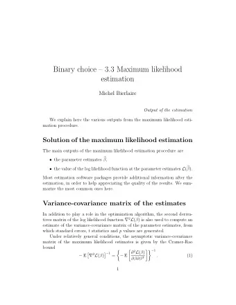
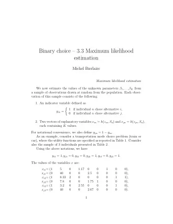
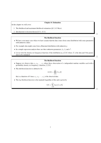
Maximum likelihood parameter estimation Maximum likelihood parameter - PDF document

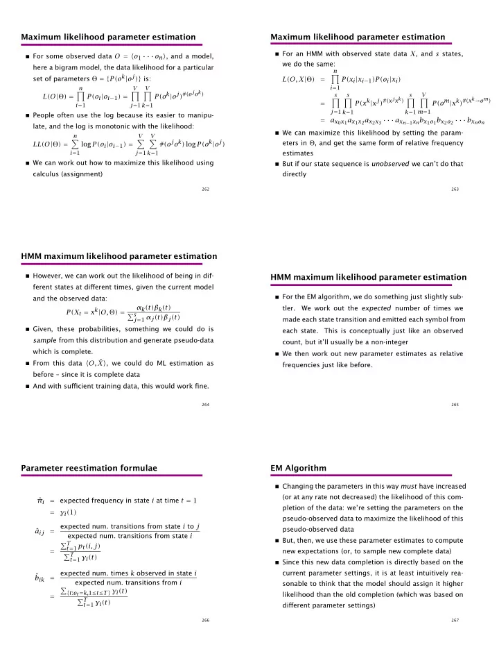
Maximum likelihood parameter estimation Maximum likelihood parameter estimation � For an HMM with observed state data X , and s states, � For some observed data O = � o 1 · · · o n � , and a model, we do the same: here a bigram model, the data likelihood for a particular n set of parameters Θ = { P(o k | o j ) } is: � L(O, X | Θ ) = P(x i | x i − 1 )P(o i | x i ) i = 1 n V V P(o k | o j ) # (o j o k ) � � � s s s V L(O | Θ ) = P(o i | o i − 1 ) = P(x k | x j ) # (x j x k ) P(o m | x k ) # (x k → o m ) � � � � = i = 1 j = 1 k = 1 j = 1 m = 1 k = 1 k = 1 � People often use the log because its easier to manipu- = a x 0 x 1 a x 1 x 2 a x 2 x 3 · · · a x n − 1 x n b x 1 o 1 b x 2 o 2 · · · b x n o n late, and the log is monotonic with the likelihood: � We can maximize this likelihood by setting the param- n V V # (o j o k ) log P(o k | o j ) � � � eters in Θ , and get the same form of relative frequency LL(O | Θ ) = log P(o i | o i − 1 ) = i = 1 j = 1 k = 1 estimates � We can work out how to maximize this likelihood using � But if our state sequence is unobserved we can’t do that calculus (assignment) directly 262 263 HMM maximum likelihood parameter estimation � However, we can work out the likelihood of being in dif- HMM maximum likelihood parameter estimation ferent states at different times, given the current model � For the EM algorithm, we do something just slightly sub- and the observed data: α k (t)β k (t) tler. We work out the expected number of times we P(X t = x k | O, Θ ) = � s j = 1 α j (t)β j (t) made each state transition and emitted each symbol from � Given, these probabilities, something we could do is each state. This is conceptually just like an observed sample from this distribution and generate pseudo-data count, but it’ll usually be a non-integer which is complete. � We then work out new parameter estimates as relative � From this data � O, ˆ X � , we could do ML estimation as frequencies just like before. before – since it is complete data � And with sufficient training data, this would work fine. 264 265 Parameter reestimation formulae EM Algorithm � Changing the parameters in this way must have increased (or at any rate not decreased) the likelihood of this com- π i ˆ = expected frequency in state i at time t = 1 pletion of the data: we’re setting the parameters on the = γ i ( 1 ) pseudo-observed data to maximize the likelihood of this expected num. transitions from state i to j pseudo-observed data a ij ˆ = expected num. transitions from state i � But, then, we use these parameter estimates to compute � T t = 1 p t (i, j) = new expectations (or, to sample new complete data) � T t = 1 γ i (t) � Since this new data completion is directly based on the current parameter settings, it is at least intuitively rea- expected num. times k observed in state i ˆ b ik = expected num. transitions from i sonable to think that the model should assign it higher � { t : o t = k, 1 ≤ t ≤ T } γ i (t) likelihood than the old completion (which was based on = � T t = 1 γ i (t) different parameter settings) 266 267

We’re guaranteed to get no worse Information extraction evaluation � Repeating these two steps iteratively gives us the EM � Example text for IE: algorithm Australian Tom Moody took six for 82 but Chris Adams � One can prove rigorously that iterating it changes the , 123 , and Tim O’Gorman , 109 , took Derbyshire parameters in such a way that the data likelihood is non- to 471 and a first innings lead of 233 . decreasing ( ?? ) � Boxes shows attempt to extract person names (correct � But we can get stuck in local maxima or on saddle points, ones in purple) though � What score should this attempt get? � For a lot of NLP problems with a lot of hidden struc- � A stringent criterion is exact match precision/recall/F 1 ture, this is actually a big problem 268 269 Precision and recall Combining them: The F measure � Precision is defined as a measure of the proportion of Weighted harmonic mean: The F measure (where F = 1 − E ): selected items that the system got right: 1 tp F = precision = α 1 P + ( 1 − α) 1 tp + fp R � Recall is defined as the proportion of the target items where P is precision, R is recall and α weights precision and recall. (Or in terms of β , where α = 1 /(β 2 + 1 ) .) that the system selected: tp recall = A value of α = 0 . 5 is often chosen. tp + fn F = 2 PR These two measures allow us to distinguish between exclud- R + P ing target items and returning irrelevant items. At break-even point, when R = P , then F = R = P They still require human-made “gold standard” judgements. 270 271 The F measure ( α = 0 . 5 ) Ways of averaging Precision Recall Arithmetic Geometric Harmonic Minimum f(x,y) 80 10 45 28.3 17.8 10 80 20 50 40.0 32.0 20 80 30 55 49.0 43.6 30 1 0.9 80 40 60 56.6 53.3 40 0.8 0.7 0.6 80 50 65 63.2 61.5 50 0.5 0.4 0.3 80 60 70 69.3 68.6 60 0.2 0.1 80 70 75 74.8 74.7 70 0 1 80 80 80 80.0 80.0 80 0.8 0.6 80 90 85 84.9 84.7 80 0 0.2 0.4 0.4 80 100 90 89.4 88.9 80 0.6 0.2 0.8 0 1 272 273

Other uses of HMMs: Information Extraction Information Extraction (Freitag and McCallum (Freitag and McCallum 1999) 1999) � IE: extracting instance of a relation from text snippets � State topology is set by hand. Not fully connected � States correspond to fields one wishes to extract, token � Use simpler and more complex models, but generally: sequences in the context that are good for identifying � Background state the fields to be extracted, and a background “noise” � Preceding context state(s) state � Target state(s) � Estimation is from tagged data (perhaps supplemented � Following context state(s) by EM reestimation over a bigger training set) � Preceding context states connect only to target state, � The Viterbi algorithm is used to tag new text etc. � Things tagged as fields to be extracted are returned 289 290 Information Extraction (Freitag and McCallum Information Extraction (Freitag and McCallum 1999) 1999) � Each HMM is for only one field type (e.g., “speaker”) � Tested on seminar announcements and corporate acqui- � Use different HMMs for each field ( bad: no real notion sitions data sets of multi-slot structure) � Performance is generally equal to or better than that of � Semi-supervised training: target words (generated only other information extraction methods by target states) are marked � Though probably more suited to semi-structured text � Shrinkage/deleted interpolation is used to generalize pa- with clear semantic sorts, than strongly NLP-oriented rameter estimates to give more robustness in the face of problems data sparseness � HMMs tend to be especially good for robustness and � Some other work has done multi-field extraction over high recall more structured data (Borkar et al. 2001) 291 292 Information extraction Information extraction: locations and speakers 0.13 0.28 � Getting particular fixed semantic relations out of text wean hall weh 5409 0.85 doherty 4623 (e.g., buyer, sell, goods) for DB filling 5409 auditorium hall 8220 0.53 � Statistical approaches have been explored recently, par- adamson hall baker conference 0.91 mellon wing <CR> place : carnegie institute ticularly use of HMMs (Freitag and McCallum 2000) : pm <CR> <UNK> room 1.0 1.0 0.30 30 in in 0.89 00 where , , <CR> the , hall � States correspond to elements of fields to extract, token 0.11 room wing 0.42 in <CR> auditorium room <CR> baker sequences in the context that identify the fields to be extracted, and background “noise” states 0.54 0.56 porter hall hall <UNK> 0.49 <UNK> room � Estimation is from labeled data (perhaps supplemented who : of < speaker with room <CR> 1.0 speak ; 5409 about by EM reestimation over a bigger training set) appointment how 0.99 0.46 0.56 � Structure learning used to find a good HMM structure dr w professor cavalier 0.99 0.56 robert stevens will seminar 0.76 that michael christel ( � The Viterbi algorithm is used to tag new text reminder 1.0 by mr l received theater speakers has artist / is additionally here 0.24 � Things tagged as within fields are returned 0.44 293 294