4CSLL5 Parameter Estimation (Supervised and Unsupervised) - - PowerPoint PPT Presentation

4CSLL5 Parameter Estimation (Supervised and Unsupervised)

4CSLL5 Parameter Estimation (Supervised and Unsupervised)

Martin Emms October 15, 2020

4CSLL5 Parameter Estimation (Supervised and Unsupervised) Outline

Unsupervised Maximum Likelihood (re-)Estimation Hidden variant of 2nd scenario The EM Algorithm Numerically worked example More realistic run of EM

4CSLL5 Parameter Estimation (Supervised and Unsupervised) Outline

The EM Algorithm

4CSLL5 Parameter Estimation (Supervised and Unsupervised) Unsupervised Maximum Likelihood (re-)Estimation Hidden variant of 2nd scenario

Hidden variable variant

Suppose you no longer see the outcome of Z; you still see the tosses of the chosen coin, but you can’t tell which it is. The data now looks like this d Z X: tosses of chosen coin H counts 1 ? H H H H H H H H T T (8H) 2 ? T T H T T T H T T T (2H) 3 ? H T H H T H H H H T (7H) 4 ? H T H H H T H H H H (8H) 5 ? T T T T T T H T T T (1H) 6 ? H H T H H H H H H H (9H) 7 ? T H H T H H H H H T (7H) 8 ? H H H H H H T H H H (9H) 9 ? H H T T T T T H T T (3H) Z is so-called hidden variable in each case

4CSLL5 Parameter Estimation (Supervised and Unsupervised) Unsupervised Maximum Likelihood (re-)Estimation Hidden variant of 2nd scenario

We still have the probability model for combinations (Z, X), with the same parameters θa, θh|a and θh|b We would still like to find values for θa, θh|a and θh|b which again maximise the probability of the observed data For each d we just know the coin-tosses Xd. Their probability is now a sum p(Xd) = p(Z = a)p(Xd|Z = a) + p(Z = b)p(Xd|Z = b) = θaθ#(d,h)

h|a

(1 − θh|a)#(d,t) + (1 − θa)θ#(d,h)

h|b

(1 − θh|b)#(d,t) and the entire data set’s probability, p(d) is the product: p(d) =

• d

p(Xd) (11) =

• d
• θaθ#(d,h)

h|a

(1 − θh|a)#(d,t) + (1 − θa)θ#(d,h)

h|b

(1 − θh|b)#(d,t) (12)

4CSLL5 Parameter Estimation (Supervised and Unsupervised) Unsupervised Maximum Likelihood (re-)Estimation Hidden variant of 2nd scenario

The ’product of sums’ problem

p(d) =

• d
• θaθ#(d,h)

h|a

(1 − θh|a)#(d,t) + (1 − θa)θ#(d,h)

h|b

(1 − θh|b)#(d,t) so can we maximise (12), repeated above? the preceding procedure of taking logs runs into a dead-end, because p(d) is no longer all products, turning into sums. Instead the log is

• d

log

• θaθ#(d,h)

h|a

(1 − θh|a)#(d,t) + (1 − θa)θ#(d,h)

h|b

(1 − θh|b)#(d,t) and there is no known way to cleverly break this down as there was before this is essentially the problem we face if we want to do parameter estimation with hidden variables – this is done widely in eg. Machine Translation and Speech Recognition. The EM or ’Expectation Maximisation’ algorithm will turn

• ut to be the solution

4CSLL5 Parameter Estimation (Supervised and Unsupervised) Unsupervised Maximum Likelihood (re-)Estimation Hidden variant of 2nd scenario

The general hidden variable set-up

before proceeding lets try to make clear the general case of a hidden variable problem You have D data items In the fully observed case, each data item d is represented by the values of a set of variables, which we’ll split into two sets zd, xd and you have a probability model – ie. formula – spelling how likely any such fully observed case is P(zd, xd; θ) where θ are all the parameters of the model In the hidden case, for each data item d you just have values on a subset of the variables xd; the other variables zd are hidden If A(z) represents the space of all possible values for the variables z, then the probability of each partial data item is P(xd; θ) =

• k∈A(z)

P(z = k, xd ; θ)

4CSLL5 Parameter Estimation (Supervised and Unsupervised) Unsupervised Maximum Likelihood (re-)Estimation The EM Algorithm

Taking stock: what kinds of thing can we calculate?

◮ parameters given visible data: we have seen illustrations where z is

known for each datum, and where finding parameter values maximising the data likelihood was easy: its relative frequencies all the way (scenario 1: 1 vis var; scenario 2: 2 vis vars, one for coin-choice, and one for the coin-tosses on whatever coin was chosen). In fact to do the parameter estimation we really just needed numbers about how often types of

• utcomes occurred.

◮ posterior probs on hidden vars: if we have all the parameters θ, for

datum d we can ’easily’ work out P(z = k|xd; θ). In our third scenario where the coin choice was hidden, for Z = a the formula is P(Z = a|Xd; θa, θh|a, θh|b) = θaθ#(d,h)

h|a

(1 − θh|a)#(d,t) θaθ#(d,h)

h|a

(1 − θh|a)#(d,t) + (1 − θa)θ#(d,h)

h|b

(1 − θh|b)#(d,t)

◮ EM methods put those two abilities to use in iterative procedures to

re-estimate parameters

4CSLL5 Parameter Estimation (Supervised and Unsupervised) Unsupervised Maximum Likelihood (re-)Estimation The EM Algorithm

EM sketch

Let’s use the notation γd(k) for P(z = k|xd) – which is something of a convention in EM methods we will describe EM for the moment as just a kind of procedure or recipe. Later we will consider how to show that the procedure does something sensible.

◮ Viterbi EM: (i) using some values for θ, for each d work out γd(k) for

each value k ∈ A(z); (ii) pick the best z = k and ’complete’ d with this value for z making a virtual complete corpus; (iii) re-estimate θ on this virtual data. If you go back to (i) and do this over and over again you would be doing what is called Viterbi EM

◮ real EM: (i) using some values for θ, for each d work out γd(k) for each

value k ∈ A(z); (ii) pretend these γd(k) are counts in a virtual corpus of completions of d; (iii) re-estimate θ on this virtual data. If you back to (i) and do this over and over again you would be doing what is called EM

4CSLL5 Parameter Estimation (Supervised and Unsupervised) Unsupervised Maximum Likelihood (re-)Estimation The EM Algorithm

EM sketch specific for scenario 3 (hidden coin choice)

◮ Viterbi EM: (i) using some values for θa, θh|a, θh|b, for each d work out

γd(k) for each value k ∈ {a, b}; (ii) pick the best Z = k and ’complete’ d with this value for Z making a virtual complete corpus; (iii) re-estimate θa, θh|a, θh|b on this virtual data. If you go back to (i) and do this over and

• ver again you would be doing what is called Viterbi EM

◮ real EM: (i) using some values for θa, θh|a, θh|b, for each d work out γd(k)

for each value k ∈ {a, b}; (ii) pretend these γd(k) are counts in a virtual corpus of completions of d; (iii) re-estimate θa, θh|a, θh|b on this virtual

• data. If you back to (i) and do this over and over again you would be

doing what is called EM

4CSLL5 Parameter Estimation (Supervised and Unsupervised) Unsupervised Maximum Likelihood (re-)Estimation The EM Algorithm

The EM algorithm

The EM algorithm is a parameter (re)-estimation procedure, which starting from some original setting of parameters θ0, generates a converging sequence

• f re-estimates:

θ0 → . . . → θn → θn+1 → . . . → θfinal where each θn goes to θn+1 by a so-called E-step, followed by a M step:

E step

generate a virtual complete data corpus by treating each incomplete data item (xd) as standing for all possible completions with values for z, (z = k, xd), weighting each by its conditional probability P(z = k|xd; θn), under current parameters θn: often this quantity is called the responsibility. Use γd(k) for P(z = k|xd).

M step

treating the ’responsibilities’ γd(k) as if they were counts, apply maximum likelihood estimation to the virtual corpus to derive new estimates θn+1.

4CSLL5 Parameter Estimation (Supervised and Unsupervised) Unsupervised Maximum Likelihood (re-)Estimation The EM Algorithm

The E step gives weighted guesses, γd(k), for each way of completing each data point. These γd(k) are then treated as counts of virtual completed data, so each data point xd is split into virtual population xd        virtual data virtual ’count’ (z = 1, xd) γd(1) : : (z = k, xd) γd(k)

4CSLL5 Parameter Estimation (Supervised and Unsupervised) Unsupervised Maximum Likelihood (re-)Estimation The EM Algorithm

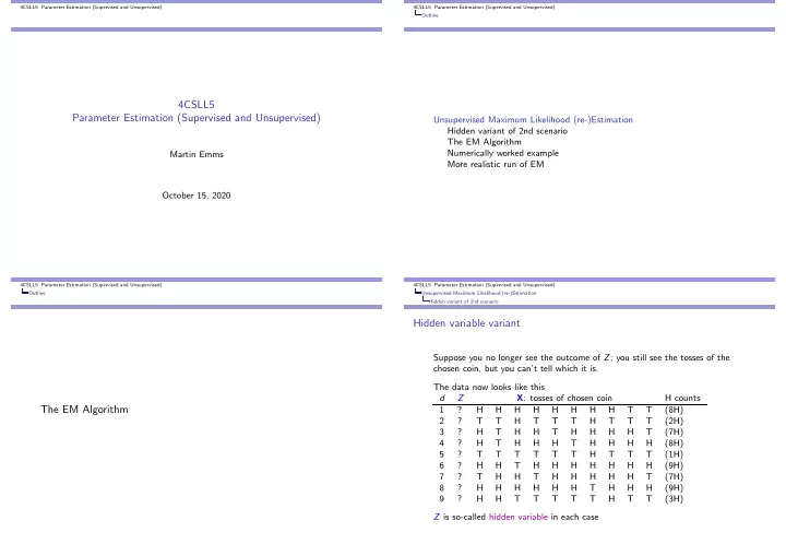
recall the observed data for our 3rd scenario, with coin-choice hidden: d Z X: tosses of chosen coin H counts 1 ? H H H H H H H H T T (8H) 2 ? T T H T T T H T T T (2H) 3 ? H T H H T H H H H T (7H) 4 ? H T H H H T H H H H (8H) 5 ? T T T T T T H T T T (1H) 6 ? H H T H H H H H H H (9H) 7 ? T H H T H H H H H T (7H) 8 ? H H H H H H T H H H (9H) 9 ? H H T T T T T H T T (3H)

4CSLL5 Parameter Estimation (Supervised and Unsupervised) Unsupervised Maximum Likelihood (re-)Estimation The EM Algorithm

E step for coin example

In the E-step you should picture each data point Xd as split into virtual population of Z = a and Z = b versions, with γd(Z) as the virtual counts 1 : X1 : (8H, 2T)

• (z = a, X1) γ1(a) = 0.88

(z = b, X1) γ1(b) = 0.12 X6 : (9H, 1T)

• (z = a, X6) γ6(a) = 0.92

(z = b, X6) γ6(b) = 0.08 X2 : (2H, 8T) (z = a, X2) γ2(a) = 0.34 (z = b, X2) γ2(b) = 0.66 X7 : (7H, 3T) (z = a, X7) γ7(a) = 0.83 (z = b, X7) γ7(b) = 0.17 X3 : (7H, 3T) (z = a, X3) γ3(a) = 0.83 (z = b, X3) γ3(b) = 0.17 X8 : (9H, 1T) (z = a, X8) γ8(a) = 0.92 (z = b, X8) γ8(b) = 0.08 X4 : (8H, 2T) (z = a, X4) γ4(a) = 0.88 (z = b, X4) γ4(b) = 0.12 X9 : (3H, 7T) (z = a, X9) γ9(a) = 0.45 (z = b, X9) γ9(b) = 0.55 X5 : (1H, 9T) (z = a, X5) γ5(a) = 0.25 (z = b, X5) γ5(b) = 0.75

1the γd(Z) numbers above assume θa = 0.5, θh|a = 0.4, θh|b = 0.3 4CSLL5 Parameter Estimation (Supervised and Unsupervised) Unsupervised Maximum Likelihood (re-)Estimation The EM Algorithm

Example calc of γ1(Z)

d = 1 : p(Z = a, HHHHHHHHTT) = 0.5 × (0.4)8 × (0.6)2 = 1.17965 × 10−4 d = 1 : p(Z = b, HHHHHHHHTT) = 0.5 × (0.3)8 × (0.7)2 = 1.60744 × 10−5 d = 1 : sum = 0.000134039 γ1(a) = p(Z = a, HHHHHHHHTT)

• z P(Z = z, HHHHHHHHTT) = 1.17965 × 10−4

sum = 0.880077 γ1(b) = p(Z = b, HHHHHHHHTT)

• z P(Z = z, HHHHHHHHTT) = 1.60744 × 10−5

sum = 0.119923

4CSLL5 Parameter Estimation (Supervised and Unsupervised) Unsupervised Maximum Likelihood (re-)Estimation The EM Algorithm

M step for coin example

In the M step you treat the γd(Z) values as if they were genuine counts and re-estimate parameters in the usual common-sense fashion based on relative frequencies. As a mental trick to help visualize you might consider all the preceding γd(Z) as multiplied by 100 – effectively each single d is being treated as split out into 100 virtual versions, with γd(Z) × 100 for each Z alternative the ’common-sense’ re-estimation of the parameters obtained this way represent a maximum likelihood estimate for any complete corpus that exhibits the same ratios as the obtained virtual corpus.

4CSLL5 Parameter Estimation (Supervised and Unsupervised) Unsupervised Maximum Likelihood (re-)Estimation The EM Algorithm

M step for coin example

For the coin scenario we can write down formulae for what the new round of estimates will be In (??), (??), (??) we had the estimation formulae for the fully observed case, making use of an indicator functions δ(d, .) – which for any given d are 1 for just one value of Z. The re-estimation formula for an M step are just these with the indicator function δ(d, .) replaced throughout by γd(.) est(θa) =

• d γd(A)

D (13) est(θh|a) =

• d γd(A)#(d, h)
• d γd(A)10

(14) est(θh|b) =

• d γd(B)#(d, h)
• d γd(B)10

(15)

4CSLL5 Parameter Estimation (Supervised and Unsupervised) Unsupervised Maximum Likelihood (re-)Estimation The EM Algorithm

’common sense’ M-step for θa, θh|a and θh|b

in case that did not persuade, here’s how to get to these re-estimation formulae by ’common sense’ based on the virtual corpus for θa, need (cnt of virtual Z = A cases)/(cnt of all virtual Z cases), ie. est(θa) =

• d γd(a)
• d γd(a) +

d γd(b) =

• d γd(a)
• d(γd(a) + γd(b)) =
• d γd(A)

D (16) for θh|a, need (cnt of H in virtual Z = a cases)/(cnt of all tosses in virtual Z = a cases), ie. est(θh|a) =

• d γd(a)#(d, h)
• d γd(a)(#(d, h) + #(d, t)) =
• d γd(a)#(d, h)
• d γd(a)10

(17) for θh|b, need (cnt of H in virtual Z = b cases)/(cnt of all tosses in virtual Z = b cases), ie. est(θh|b) =

• d γd(b)#(d, h)
• d γd(b)(#(d, h) + #(d, t)) =
• d γd(b)#(d, h)
• d γd(b)10

(18)

4CSLL5 Parameter Estimation (Supervised and Unsupervised) Unsupervised Maximum Likelihood (re-)Estimation The EM Algorithm

Properties of EM re-estimation

EM starts with some setting θ0 of the parameters and one E-M cycle takes one setting θn into another θn+1. the data gets likelier over the iterations P(d; θn) ≤ P(d; θn+1) because the data cannot just get likelier and likelier, the procedure converges to a final setting θfinal so whatever values θ0 you start with, running the algorithm will give you better values θfinal

4CSLL5 Parameter Estimation (Supervised and Unsupervised) Unsupervised Maximum Likelihood (re-)Estimation The EM Algorithm

some provisos though ...

◮ Caveat One: there may be many local maxima, so there is no guarantee

that the re-estimation will converge to the best values

◮ Caveat Two: if the data set d is rather small the derived parameters may

fit fresh data only poorly – this the classic over-fitting problem.

◮ Caveat Three: it will be prohibitively expensive to calculate all γd(k) if the

set A(z) of the possible values of z is exponentially big. This does not apply to our hidden coin choice scenario – size of A(z) is 2 – but definitely applies to applications we are going to look at (eg. in Machine Translation and Speech Recognition) and requires algorithic ingenuity to make it still work.

4CSLL5 Parameter Estimation (Supervised and Unsupervised) Unsupervised Maximum Likelihood (re-)Estimation Numerically worked example

A numerically worked example

To keep things manageable on slides lets suppose a minute data set d Z X: tosses of chosen coin 1 ? H H 2 ? T T looks like having A be entirely biased one way, and B entirely the other will give maximum prob to this. The outcomes when EM is run from start θa = 0.5, θh|a = 0.75 and θh|b = 0.5 is: θa θh|a θh|b logprob prob 0.5 0.75 0.5

• 3.97763

0.0634766 0.446154 0.775862 0.277778

• 3.36722

0.0969094 0.467361 0.922972 0.128866

• 2.59395

0.165632 0.49254 0.993083 0.0214144

• 2.08205

0.236179 : : : : : 0.5 1

• 2

0.25 so EM finds the intuitive solution. Next few slides trace the first iteration of the algorithm

4CSLL5 Parameter Estimation (Supervised and Unsupervised) Unsupervised Maximum Likelihood (re-)Estimation Numerically worked example

Let Xd be the coin toss outcomes for a particular trial. The probability of the version where the chosen coin was A is P(Z = a, Xd) = P(Z = a) × P(h|a)#(d,h) × P(t|a)#(d,t) = θa × θ#(d,h)

h|a

× θ#(d,t)

t|a

and likewise the probability of the version where the chosen coin was B is given by P(Z = b, Xd) = P(Z = b) × P(h|b)#(d,h) × P(t|b)#(d,t) = θb × θ#(d,h)

h|b

× θ#(d,t)

t|b

and from these joint probability formula the conditional probabilities for the hidden variable will be: P(Z = a|Xd) = P(Z = a, Xd)

• k P(Z = k, Xd)

P(Z = b|Xd) = P(Z = b, Xd)

• k P(Z = k, Xd)

4CSLL5 Parameter Estimation (Supervised and Unsupervised) Unsupervised Maximum Likelihood (re-)Estimation Numerically worked example

On the particular data set at hand the joint probability formulae are particularly simple P(Z = a, X1) = θa × (θh|a)2 P(Z = b, X1) = θb × (θh|b)2 P(Z = a, X2) = θa × (θt|a)2 P(Z = b, X2) = θb × (θt|b)2 and thus the formulae for γd(Z) are: γ1(a) = θa × (θh|a)2 θa × (θh|a)2 + θb × (θh|b)2 γ1(b) = θb × (θh|b)2 θa × (θh|a)2 + θb × (θh|b)2 γ2(a) = θa × (θt|a)2 θa × (θt|a)2 + θb × (θt|b)2 γ2(b) = θb × (θt|b)2 θa × (θt|a)2 + θb × (θt|b)2

4CSLL5 Parameter Estimation (Supervised and Unsupervised) Unsupervised Maximum Likelihood (re-)Estimation Numerically worked example

To carry out an EM estimation of the parameters given the data we need some initial setting of the parameters. We will suppose this is: θa = 1 2, θb = 1 2, θh|a = 3 4, θt|a = 1 4, θh|b = 1 2, θt|b = 1 2 ITERATION 1 For each piece of data have to first compute the conditional probabilities of the hidden variable given the data: d = 1 : p(Z = A, HH) = 0.5 × 0.75 × 0.75 = 0.28125 d = 1 : p(Z = B, HH) = 0.5 × 0.5 × 0.5 = 0.125 d = 1 :→ sum = 0.40625 d = 1 :→ γ1(A) = 0.692308 d = 1 :→ γ1(B) = 0.307692 d = 2 : p(Z = A, TT) = 0.5 × 0.25 × 0.25 = 0.03125 d = 2 : p(Z = B, TT) = 0.5 × 0.5 × 0.5 = 0.125 d = 2 :→ sum = 0.15625 d = 2 :→ γ2(A) = 0.2 d = 2 :→ γ2(B) = 0.8

4CSLL5 Parameter Estimation (Supervised and Unsupervised) Unsupervised Maximum Likelihood (re-)Estimation Numerically worked example

Armed with these γ values we now treat each data item Xd as if it splits into two versions, one filling out Z as a, and with ’count’ γd(a), and one filling out Z as b, and with ’count’ γd(b). X1 : (2H, 0T) (z = a, X1) γ1(a) = 0.692308 (z = b, X1) γ1(b) = 0.307692 X2 : (0H, 2T)

• (z = a, X2) γ2(a) = 0.2

(z = b, X2) γ2(b) = 0.8

4CSLL5 Parameter Estimation (Supervised and Unsupervised) Unsupervised Maximum Likelihood (re-)Estimation Numerically worked example

X1 : (2H, 0T) (z = a, X1) γ1(a) = 0.692308 (z = b, X1) γ1(b) = 0.307692 X2 : (0H, 2T)

• (z = a, X2) γ2(a) = 0.2

(z = b, X2) γ2(b) = 0.8 We then go through this virtual corpus accumulating counts of certain kinds of

• event. For events of hidden variable being Z = a and Z = b we get

E(A) = γ1(a) + γ2(a) = 0.692308 + 0.2 = 0.892308 E(B) = γ1(b) + γ2(b) = 0.307692 + 0.8 = 1.10769 Then we need to go through the Z = a cases and count types of coin toss, and likewise for Z = b cases E(A, H) =

d γd(a)#(d, h) = (0.692308 × 2 + 0.2 × 0) = 1.38462

E(A, T) =

d γd(a)#(d, t) = (0.692308 × 0 + 0.2 × 2) = 0.4

E(B, H) =

d γd(b)#(d, h) = (0.307692 × 2 + 0.8 × 0) = 0.615385

E(B, T) =

d γd(b)#(d, t) = (0.307692 × 0 + 0.8 × 2) = 1.6

4CSLL5 Parameter Estimation (Supervised and Unsupervised) Unsupervised Maximum Likelihood (re-)Estimation Numerically worked example

re-estimating θa and θb

Then from these ’expected’ counts we re-estimate parameters est(θa) = E(A)/2 = 0.892308/2 = 0.446154 est(θb) = E(B)/2 = 1.10769/2 = 0.553846 Note the denominator 2 in the re-estimation formula for θa. We could have written the denominator as E(A) + E(B), but this is

• d

γd(a) +

• d

γd(b) =

• d

[γd(a) + γd(b)] =

• d

[1] = 2

4CSLL5 Parameter Estimation (Supervised and Unsupervised) Unsupervised Maximum Likelihood (re-)Estimation Numerically worked example

re-estimating θh|a

est(θh|a) = E(A, H)/

• X

[E(A, X)] = 1.38462/(1.38462 + 0.4) = 1.38462/1.78462 = 0.775862 est(θt|a) = E(A, T)/

• X

[E(A, X)] = 0.4/(1.38462 + 0.4) = 0.4/1.78462 = 0.224138

4CSLL5 Parameter Estimation (Supervised and Unsupervised) Unsupervised Maximum Likelihood (re-)Estimation Numerically worked example

re-estimating θh|b

est(θh|b) = E(B, H)/

• X

[E(B, X)] = 0.615385/(0.615385 + 1.6) = 0.615385/2.21538 = 0.277778 est(θt|b) = E(B, T)/

• X

[E(B, X)] = 1.6/(0.615385 + 1.6) = 1.6/2.21538 = 0.722222

4CSLL5 Parameter Estimation (Supervised and Unsupervised) Unsupervised Maximum Likelihood (re-)Estimation Numerically worked example

the above traced through how the 2nd row of the table below comes from the first. θa θh|a θh|b logprob prob 0.5 0.75 0.5

• 3.97763

0.0634766 0.446154 0.775862 0.277778

• 3.36722

0.0969094 0.467361 0.922972 0.128866

• 2.59395

0.165632 0.49254 0.993083 0.0214144

• 2.08205

0.236179 : : : : : 0.5 1

• 2

0.25 In the end it converges to θa = 0.5, θh|a = 1, θh|b = 0. also tracked in the table is the increasing prob of the data, and log-prob

4CSLL5 Parameter Estimation (Supervised and Unsupervised) Unsupervised Maximum Likelihood (re-)Estimation More realistic run of EM

More realistic run of EM

recall the data we had for our 2nd scenario, with the coin-choice observed: d Z X: tosses of chosen coin H counts 1 A H H H H H H H H T T (8H) 2 B T T H T T T H T T T (2H) 3 A H T H H T H H H H T (7H) 4 A H T H H H T H H H H (8H) 5 B T T T T T T H T T T (1H) 6 A H H T H H H H H H H (9H) 7 A T H H T H H H H H T (7H) 8 A H H H H H H T H H H (9H) 9 B H H T T T T T H T T (3H) recall supervised estimation gave: θa = 0.66, θh|a = 0.8, θh|b = 0.2

4CSLL5 Parameter Estimation (Supervised and Unsupervised) Unsupervised Maximum Likelihood (re-)Estimation More realistic run of EM

More realistic run of EM continued

here’s an outcome of running EM treating Z as hidden θa θh|a θh|b logprob prob 0.5 0.4 0.3

• 101.033

3.85587e-31 0.698501 0.70713 0.351806

• 77.3507

5.18952e-24 0.666619 0.793432 0.213219

• 73.2502

8.90206e-23 0.66705 0.799293 0.200725

• 73.2201

9.08992e-23 0.667134 0.799354 0.200453

• 73.2201

9.08999e-23 no further change these are very close to the numbers obtained when Z was not hidden. On this data set also the final outcome is not very dependent on the initial values