Lecture 4: Problem solving as search: Solution = a finite sequence - - PowerPoint PPT Presentation

Lecture 4:
 Heuristic search
 and local search

• Prof. Julia Hockenmaier

juliahmr@illinois.edu

• http://cs.illinois.edu/fa11/cs440
• CS440/ECE448: Intro to Artificial Intelligence

Tuesdayʼs key concepts

Problem solving as search:

Solution = a finite sequence of actions


• State graphs and search trees

Which one is bigger/better to search?


• Systematic (blind) search algorithms

Breadth-first vs. depth-first; properties?
 


• 2

CS440/ECE448: Intro AI

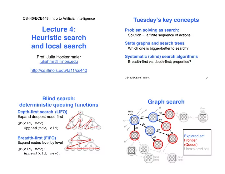
Blind search: 
 deterministic queuing functions

Depth-first search (LIFO)

• Expand deepest node first

QF(old, new): 
 Append(new, old)


• Breadth-first (FIFO)

Expand nodes level by level QF(old, new): 
 Append(old, new);

• A

B C D G H J I F E A B C D G H J I F E

Graph search

Initial state a2 a1 a3

Explored set Frontier (Queue) Unexplored set

…. Goal state

Goal state ….

Goal state …. b3 c5 b4 b1 b2

Todayʼs key questions

How can we find the optimal solution?

We need to assign values to solutions
 


How can we find a better solution if we can only foresee the effect (=value) of the next action?

This is local search.

• 5

CS440/ECE448: Intro AI

Informed 
 (heuristic) search

Considering the cost of solutions

We may not just want to find any solution,
 but the cheapest solution, if:

– Each action has a (positive, finite) cost – Some solutions may be cheaper than others
 


• 7

CS440/ECE448: Intro AI

Heuristic search: priority queue


 Heuristic search algorithms sort the nodes

• n the queue according to a cost function: 

• QF(a,b): 


sort(append(a,b), CostFunction)


• The cost function is an estimate of the true cost.

Nodes with the lowest estimated cost have 
 the highest priority.

8

Heuristic graph search

9 SEARCH(Problem P, Queuing Function QF):
 local: n, q, e; 
 q ! new List(Initial_State(P));
 Loop:
 if q == () return failure;
 n ! Pop(q);
 if n solves P return n;
 add n.STATE to e 
 for m in Expand(n):
 if m is not in e or q:
 q ! QF(q,{m}); /*NEW: we want to find the cheapest goal!*/ 
 else if m.STATE in q with higher cost:


• q ! replace(q, m.STATE, m);


end

Cost from root to node: g(n)

g*(n): Minimum cost from root to n

g*(n) is the sum of the costs for each action 
 from the root to node n. This requires a cost function for actions

g(n): Computable approximation to g*(n)


For trees: g(n) == g*(n)

10

CS440/ECE448: Intro AI

Uniform-cost search

Sort the queue by path cost g(n): First expand the node with lowest g(n)

• QF(a,b): sort(Append(a,b), g)

11

CS440/ECE448: Intro AI

Uniform-cost search illustrated

CS440/ECE448: Intro AI

12 S g = 0 F g = 99 B g = 278 R g=80 P g = 177

99 211 80 97 101 S:0 [R:80, F:99] R:80 [F:99, P:177] F:99 [P:177, B:310] P:177 [B:278, B:310] B:278 [B:310]

1 2 3 4 5

Properties of 
 uniform-cost search

Complete if b is finite, and each action has positive (non-zero) cost 


(gets stuck in loops of zero-cost actions)


Optimal.

• Time and space complexity similar to

breadth-first search if costs are uniform

(possibly much worse otherwise)

13

CS440/ECE448: Intro AI

}

g*(n)

} ???

How close are we to the goal?

14

I

Initial state

n Node n G Goal state

Cost from node to goal: h(n)

h*(n): the minimum cost from n to any goal


h*(n) is generally unknown

h(n): computable approximation to h*


h(n) is called the heuristic function

• 15

CS440/ECE448: Intro AI

} h*(n)

n G

Greedy best-first search

Sort the queue by heuristic function h(n): First expand the node with lowest h(n)

• QF(a,b): sort(Append(a,b), h)

• Problem: This ignores g(n)

16

CS440/ECE448: Intro AI

Properties of 
 greedy best-first search

Similar to DFS: Tree-search version is incomplete. Graph-search version is complete 
 in finite state spaces. Both are not optimal.

• Worst-case time and space complexity

similar to DFS 


(actual complexity depends on h)

17

CS440/ECE448: Intro AI

}

g*(n)

} h*(n)

Total cost: f*(n)

18

I

Initial state

n Node n G Goal state f*(n) = g*(n) + h*(n) f*(n) is the lowest cost solution from the initial state to a goal constrained through n

}

g(n)

} h(n)

Total estimated cost: f(n)

19

I

Initial state

n Node n G Goal state f(n) = g(n) + h(n) f(n) approximates the lowest cost solution from the initial state to a goal constrained through n

A* search

Sort the queue by total estimated cost f(n): First expand the node with lowest f(n)

• QF(a,b): sort(Append(a,b), f)
• 20

CS440/ECE448: Intro AI

Properties of A* search

A* is complete if b is finite, and each action has positive (non-zero) cost 


• Its complexity depends on the heuristic

function h(n)

• Is A* optimal?

21

CS440/ECE448: Intro AI

Tree-search A* is optimal if…

…h(n) is an admissible heuristic Admissible heuristics never overestimate
 the future cost.


• Definition

h(n) is admissible: !n " nodes: h(n) # h*(n) 


• 22

Tree-search A* is optimal 
 if h(n) is admissible

In tree-search: g(n) = g*(n) If n is a goal: f(n) = f*(n)

The goal that is returned is the cheapest on the queue!

If n is not a goal: f(n) ≤ f*(n) g(n) + h(n) ≤ g*(n) + h*(n)

f*(n): true cost of cheapest goal that can be reached from n. 


• If gno is a non-optimal goal, and nopt is an ancestor
• f the optimal goal gopt: f(nopt) ≤ f(gopt) < f(gno)

nopt will be explored first!

• 23

Confused? This is

• ptional

material

Graph-search A* is optimal if…

…h(n) is monotonic (=consistent)

Monotonic heuristics obey the triangle inequality: Going from n to the goal via nʼ is at least as expensive as going from n to the goal.

• !n!n’ " nodes,

!a " actions with a(n)$n’ h(n) # cost(n, a, n’) + h(n’)


• NB.: every monotonic heuristic is also admissible

24 n

nʼ cost(n, a, nʼ)

G

h(n) h(nʼ)

Confused? This is optional material

Graph-search A* is optimal if…

…h(n) is monotonic (=consistent)

h(n) # cost(n, a, n’) + h(n’)

• Proof sketch:
• 1. If h is monotonic, the values of f(n) along any

path are non-decreasing. (true by definition)

• 2. When n is expanded, g(n) = g*(n)

[we have found the cheapest path to n.] Thus, sorting by f finds the cheapest goal first

25

Confused? This is optional material

Possible Heuristic Functions

Often simplify by relaxing some constraint

• h1: 3

h2 (8-puzzle): 
 count # tiles out of place h3 (route-finding): 
 sum Manhattan metric distances

• Uniform-cost: huniform-cost = 0

26

Given: A1* with heuristic function h1
 and A2* with heuristic function h2

• Both A1* and A2* are admissible
• A1* is more informed than A2* iff 


for all non-goal nodes n h1(n) > h2(n)

• “More informed”: “guaranteed not to search more”
• Informed heuristics

27

Local search

Motivation for local search

How can we find the goal when:


• we canʼt keep a queue? 


(because we donʼt have the memory) 


• we donʼt want to keep a queue?


(because we just need to find the goal state, )

• we canʼt enumerate the next actions?


(because thereʼs an infinite number)


• Local search algorithms:

Consider only the current node 
 and the next action

• Also useful for optimization:

finding the best state according to
 an objective function

30

CS440/ECE448: Intro AI

8-queens

31

CS440/ECE448: Intro AI

8-queens by local search

Initial state: A board with 8 queens, one in each column. (we use a complete-state formulation).

• Action: Move one queen to another square

in its column.

• Heuristic function (score): 


How many queens attack each other?

• 32

CS440/ECE448: Intro AI

Possible successor states

14 18 17 15 14 18 14 14 14 14 14 12 16 12 13 16 17 14 18 13 14 17 15 18 15 13 15 13 12 15 15 13 15 12 13 14 14 14 16 12 14 12 12 15 16 13 14 12 14 18 16 16 16 14 16 14

33

CS440/ECE448: Intro AI

If queen in first column moves here, score = 15 The best next states

The state space landscape:
 minimizing cost…

34

CS440/ECE448: Intro AI

state space cost goal state current state

…or maximizing 
 an objective function

35

CS440/ECE448: Intro AI

state space

• bjective

function = −cost goal state current state

The state space landscape

36

CS440/ECE448: Intro AI

state space

• bjective

function global maximum plateau local maximum current state

Goal: reaching the global maximum

37

CS440/ECE448: Intro AI

state space

• bjective

function global maximum plateau local maximum current state You win! HillClimb(Problem P): local:n /*current node*/
 n ! InitialState(P); Loop: n’ ! highestValueNeighborOf(n); /* Are we at the peak yet? */ if n’.VALUE ≤ n.VALUE return n; else n = n’ /* Keep climbing up to n’ */ end

Generic Search Function

Hill-climbing search

local maximum#!@*!

Problem: local maxima are difficult to avoid

39

CS440/ECE448: Intro AI

state space

• bjective

function global maximum plateau current state

A local maximum for 8 queens

40

CS440/ECE448: Intro AI

local maximum

#!@*!

Problem: plateaus are difficult
 to navigate

41

CS440/ECE448: Intro AI

state space

• bjective

function global maximum plateau current state

Ideal case:
 Convex optimization

42

CS440/ECE448: Intro AI

state space

• bjective

function global maximum

When the objective function is convex, 
 search/optimization becomes vastly simplified.

Dealing with local maxima

Random restart hill-climbing: k trials starting from random positions

• k-best (beam) hill climbing:

Pursue k trials in parallel; only keep the k best successors at each time step

• Simulated annealing:

Accept downhill moves with non-zero prob.

43

CS440/ECE448: Intro AI

RandomRestartHillClimb(Problem P): local:n, nMax; /* current best node*/
 For r = 1 … R: /* try R times*/ n ! RandomInitialState(P); nMax ! n; Loop (climb): n’ ! highestValueNeighborOf(n); if n’.VALUE > nMax.VALUE nMax ! n’; if n’.VALUE > n.VALUE n ! n’; else exit Loop; return nMax;

Generic Search Function

Random restart 
 hill-climbing search

K-bestHillClimb(Problem P, int k): local: N = Array[k] /*vector of K node*/ for i = 0…k-1: N[i] ! RandomInitialState(P); N ! sort(N) Loop: nMax = N[0]; local: N’ = Array[k], M = Array[2k] for i = 0…k-1: N’[i] ! highestValueNeighborOf(n[i]);
 M ! sort(append(N, N’)); N ! M[0…k-1]; if N[0].VALUE ≤ nMax.VALUE return nMAx; end

Generic Search Function

k-best (beam) hill climbing

Generic Search Function

Simulated annealing

A version of stochastic hill-climbing: go downhill with non-zero probability pdown

• pdown depends on step size:

pdown is greater for smaller steps.

• pdown depends on current temperature:

pdown is greater at high temperature. Temperature is a function of time: Start with high temperature, lower gradually.

• Computing pdown

∆Value: neighbor.VALUE – this.VALUE In a downhill move, ∆Value is negative.

• Temperature:

We define temperature to be a decreasing function of time.

• pdown = e∆Value/Temperature

47

CS440/ECE448: Intro AI

Temperature = 10

48

CS440/ECE448: Intro AI

0.1 0.2 0.3 0.4 0.5 0.6 0.7 0.8 0.9 1

• 50
• 40
• 30
• 20
• 10

pdown Value T=10

0.1 0.2 0.3 0.4 0.5 0.6 0.7 0.8 0.9 1

• 50
• 40
• 30
• 20
• 10

pdown Value T=10 T=5

Temperature = 5

49

CS440/ECE448: Intro AI

0.1 0.2 0.3 0.4 0.5 0.6 0.7 0.8 0.9 1

• 50
• 40
• 30
• 20
• 10

pdown Value T=10 T=5 T=2

Temperature = 2

50

CS440/ECE448: Intro AI

0.2 0.4 0.6 0.8 1

• 50
• 40
• 30
• 20
• 10

pdown Value T=10 T=5 T=2 T=0.0001

Temperature = 0.0001

51

CS440/ECE448: Intro AI

SimAnnealing(Problem P): local:n 
 n ! InitialState(P); For time = 1 to ∞ do: Temperature = temp(time); if Temperature == 0 return n; n’ ! randomNeighborOf(n); ∆Value = n’.VALUE - n.VALUE; if ∆Value > 0 n ! n’ else n ! n’ with prob. e∆Value/Temperature end

Generic Search Function

Simulated annealing

To conclude…

Todayʼs key concepts

Heuristic search: Actions and solutions have costs Heuristic function: estimate of future cost Uniform cost, best-first, A*

• Local search:

Agent only sees the next steps. Features of the state space landscape Hill-climbing, random restart, beam, simulated annealing

Your tasks

Reading: Chapter 3.5, Chapter 4.1

• Compass quiz:

Up at 2pm

• Assignments:


MP 1 will go out this afternoon.

55

CS440/ECE448: Intro AI