Lecture 10: Stereo databases Build a shape-based object detector - - PDF document

lecture 10 stereo
SMART_READER_LITE
LIVE PREVIEW

Lecture 10: Stereo databases Build a shape-based object detector - - PDF document

Grad student extension ideas for problem set 2 Implement textons approach for texture recognition [Leung & Malik] Possible data sources: Vistex, Curet Lecture 10: Stereo databases Build a shape-based object detector using the


slide-1
SLIDE 1

Lecture 10: Stereo

Tuesday, Oct 2

Grad student extension ideas for problem set 2

  • Implement textons approach for texture

recognition [Leung & Malik]

– Possible data sources: Vistex, Curet databases

  • Build a shape-based object detector using

the generalized Hough transform

  • Clustering approach to video shot

boundary detection

  • Build a deformable contour tracker

Exam

  • Next Tuesday, Oct 9, in class
  • Bring one handwritten 8.5 x 11”, one-sided

sheet with any notes

  • Closed book/laptop/calculator

Review all material covered so far

  • Image formation

– Perspective, orthographic projection properties, equations, effects – Pinhole cameras – Thin lens – Field of view, depth of field

  • Color

– BRDF – Spectral power distribution – Color mixing – Color matching – Color spaces – Human perception

  • Binary image analysis

– Histograms and thresholding – Connected components – Morphological operators – Region properties and invariance – Distance transform, Chamfer distance

  • Filters

– Application/effects of – Convolution properties – Noise models – Mean, median, Gaussian, derivative filters – Separability

  • Edges, pyramids, sampling

– Image gradients – Effects of noise – Derivative of Gaussian, Laplacian filters – Canny edge detection – Corner detection – Sampling and aliasing – Pyramids – construction and applications

  • Texture

– Analysis vs. synthesis – Representations

  • Grouping

– Gestalt principles – Clustering: agglomerative, k-means, mean shift, graph-based – Graphs and affinity matrices

  • Fitting

– Hough transform – Generalized Hough transform – Least squares – Incremental line fitting, k-means – Robust fitting: RANSAC, M-estimators – Deformable contours, energy functions

  • Stereo vision

Outline

  • Brief review of deformable contours
  • Fundamentals of stereo vision
  • Epipolar geometry

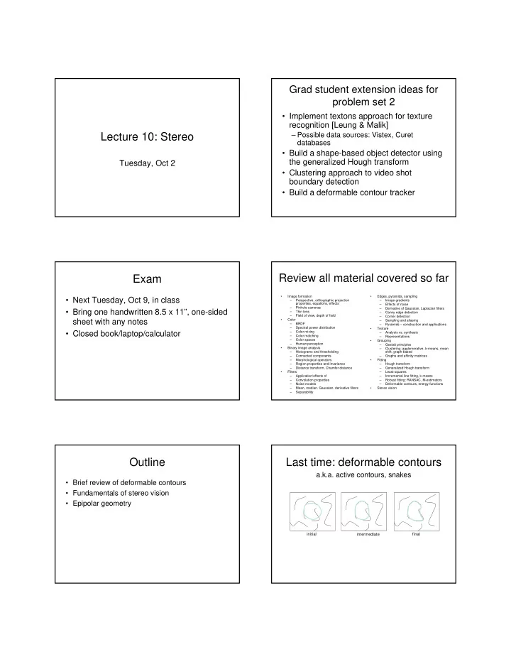
Last time: deformable contours

initial intermediate final

a.k.a. active contours, snakes

slide-2
SLIDE 2

Snake energy function

The total energy of the current snake defined as

ex in total

E E E + =

Internal energy encourages smoothness

  • r any particular shape

Internal energy incorporates prior knowledge about object boundary, which allows a boundary to be extracted even if some image data is missing External energy encourages curve onto image structures (e.g. image edges)

We will want to iteratively minimize this energy for a good fit between the deformable contour and the target shape in the image

Discrete energy terms

  • If the curve is represented by n points

Elasticity, Tension; Want to favor close points Stiffness Curvature; Want to favor smoothly shaped curve (not corners)

1 ) , ( − = = n i y x

i i i

K ν

2

1 i i

v ds d ν ν − ≈

+ 1 1 1 1 2 2

2 ) ( ) (

− + − +

+ − = − − − ≈

i i i i i i i

ds d ν ν ν ν ν ν ν ν

− = − + +

+ − + − =

1 2 1 1 2 1

| 2 | | |

n i i i i i i in

E ν ν ν β ν ν α

Discrete energy terms

  • An external energy term for a (discrete)

snake based on image edge

2 1 2

| ) , ( | | ) , ( |

i i y n i i i x ex

y x G y x G E

− =

+ − =

Energy minimization

  • Many algorithms proposed to fit

deformable contours

– Greedy search – Gradient descent – Dynamic programming (for 2d snakes)

Problems with snakes

  • Depends on number and spacing of control

points

  • Snake may oversmooth the boundary
  • Not trivial to prevent curve self intersecting
  • Cannot follow topological changes of objects

Problems with snakes

  • May be sensitive to initialization, get stuck

in local minimum

  • Accuracy (and computation time) depends
  • n the convergence criteria used in the

energy minimization technique

slide-3
SLIDE 3

Problems with snakes

  • External energy: snake does not really “see”
  • bject boundaries in the image unless it gets very

close to it.

image gradients are large only directly on the boundary

I ∇

Depth unavailable in single views

Optical center

P1 P2 P1’=P2’

What cues can indicate 3d shape?

Shading

[Figure from Prados & Faugeras 2006]

Focus/Defocus

[Figure from H. Jin and P. Favaro, 2002]

Texture

[From A.M. Loh. The recovery of 3-D structure using visual texture patterns. PhD thesis]

slide-4
SLIDE 4

Motion

Figures from L. Zhang http://www.brainconnection.com/teasers/?main=illusion/motion-shape

Estimating scene shape

  • Shape from X: Shading, Texture, Focus, Motion…
  • Stereo:

– shape from motion between two views – infer 3d shape of scene from two (multiple) images from different viewpoints

Accommodation and focus

The lens modifies the image focus by adjusting its focal length.

Fixation, convergence

Fixation, convergence

From Palmer, “Vision Science”, MIT Press

Human stereopsis: disparity

Disparity occurs when eyes verge on one object;

  • thers appear at different

visual angles

slide-5
SLIDE 5

Disparity: d = r-l = D-F. d=0

Human stereopsis: disparity

Adapted from M. Pollefeys

Random dot stereograms

  • Julesz 1960: Do we identify local

brightness patterns before fusion (monocular process) or after (binocular)?

  • To test: pair of synthetic images obtained

by randomly spraying black dots on white

  • bjects

Random dot stereograms

Forsyth & Ponce

Random dot stereograms Random dot stereograms

From Palmer, “Vision Science”, MIT Press

Random dot stereograms

  • When viewed monocularly, they appear random;

when viewed stereoscopically, see 3d structure.

  • Conclusion: human binocular fusion not directly

associated with the physical retinas; must involve the central nervous system

  • Imaginary “cyclopean retina” that combines the

left and right image stimuli as a single unit

slide-6
SLIDE 6

Generating a random dot stereogram

http://www.wellesley.edu/CS/LiDPC/OnParallaxis/Braunl.paper20.html

Autostereograms

Images from magiceye.com

Exploit disparity as depth cue using single image (Single image random dot stereogram, Single image stereogram)

Images from magiceye.com

Autostereograms

Images from magiceye.com

Autostereograms

Stereo photography and stereo viewers

Invented by Sir Charles Wheatstone, 1838

Image courtesy of fisher-price.com

Take two pictures of the same subject from two slightly different viewpoints and display so that each eye sees only

  • ne of the images.

http://www.johnsonshawmuseum.org

slide-7
SLIDE 7

http://www.johnsonshawmuseum.org

Public Library, Stereoscopic Looking Room, Chicago, by Phillips, 1923

http://www.well.com/~jimg/stereo/stereo_list.html

Stereo in machine vision systems

Left : The Stanford cart sports a single camera moving in discrete increments along a straight line and providing multiple snapshots of

  • utdoor scenes

Right : The INRIA mobile robot uses three cameras to map its environment

Forsyth & Ponce

Stereo

  • Main issues

– Geometry: what information is available, how do the camera views relate? – Correspondences: what feature in view 1 corresponds to feature in view 2? – Triangulation, reconstruction: inference in presence of noise

Multi-view geometry

Slide credit: T. Darrell

slide-8
SLIDE 8

Camera parameters

Camera frame

Intrinsic: Image coordinates relative to camera Pixel coordinates Extrinsic: Camera frame Reference frame

World frame

  • Extrinsic params: rotation matrix and translation vector
  • Intrinsic params: focal length, pixel sizes (mm), image center

point, radial distortion parameters

Geometry for a simple stereo system

  • First, assuming parallel optical axes,

known camera parameters:

  • Parameters in this case:

– Camera centers (Ol, Or) – Focal length (f) – Baseline (T)

Geometry for a simple stereo system

  • First, assuming parallel optical axes,

known camera parameters:

Similar triangles (pl, P, pr) and (Ol, P, Or) T + xl – xr = T

  • Z – f Z

Z = f T/d where d = xr – xl

Geometry for a simple stereo system

Stereo constraints

  • Given p in left image, where can

corresponding point p’ be?

slide-9
SLIDE 9

Stereo constraints

  • Given p in left image, where can

corresponding point p’ be?

Stereo constraints

Adapted from M. Pollefeys, UNC

  • Epipolar Plane
  • Epipoles
  • Epipolar Lines
  • Baseline

Epipolar geometry

Now the optical axes are not necessarily parallel.

Epipolar geometry

  • Baseline: line joining the camera centers
  • Epipole: point of intersection of baseline with the

image plane

  • Epipolar plane: plane containing baseline
  • Epipolar line: intersection of epipolar plane with

the image plane

  • All epipolar lines intersect at the epipole
  • An epipolar plane intersects the left and right

image planes in epipolar lines

  • Potential matches for p have to lie on the corresponding

epipolar line l’.

  • Potential matches for p’ have to lie on the corresponding

epipolar line l.

Slide credit: M. Pollefeys

Epipolar constraint Epipolar constraint example

slide-10
SLIDE 10

Example: converging cameras

Figure from Hartley & Zisserman

As position of 3d point varies, epipolar lines “rotate” about the baseline

Example: motion parallel with image plane

Figure from Hartley & Zisserman

Example: forward motion

Figure from Hartley & Zisserman

e e’

Epipole has same coordinates in both images. Points move along lines radiating from e: “Focus of expansion”

Reconstruction by triangulation

  • Assuming intrinsic and extrinsic parameters are

known, compute 3d location of point P from projections p and p’:

  • Intersect rays R = Op and R’ = O’p’.

p p’ P O O’

Reconstruction by triangulation

  • Assuming intrinsic and extrinsic parameters are

known, compute 3d location of point P from projections p and p’:

  • Intersect rays R = Op and R’ = O’p’.

But, in practice, parameters and image locations only approximately known…

p p’ P O O’

Triangulation with non- intersecting rays (1)

Construct line segment perpendicular to R and R’ that intersects both rays Midpoint of this segment is closest point to the two rays, use as P estimate of scene point

slide-11
SLIDE 11

Triangulation with non- intersecting rays (2)

Estimate scene point Q as the point that minimizes summed squared distance between p and q, and p’ and q’ (non-linear least squares, iterative, not closed form)

Next

  • 3d reconstruction
  • Building stereo algorithms

– correspondences