Outline Last lecture: stereo reconstruction with calibrated - PDF document

Outline • Last lecture: – stereo reconstruction with calibrated cameras – non-geometric correspondence constraints Lecture 12: Multi-view • Homogeneous coordinates, projection matrices geometry / Stereo III • Camera calibration • Weak calibration/self-calibration Tuesday, Oct 23 – Fundamental matrix – 8-point algorithm CS 378/395T Prof. Kristen Grauman Review: stereo with calibrated cameras Review: the essential matrix [ ] Vector p’ in ( ) ′ ⋅ × = second coord. p T R p 0 sys. has [ ] ′ ⋅ = coordinates Rp’ p T R p 0 x in the first one. [ ] = Let E T R x Τ p ′ = p E 0 E is the essential matrix , which relates corresponding image points in both cameras, given the rotation and translation between their coordinate systems. Camera-centered coordinate systems are related by known rotation R and translation T . 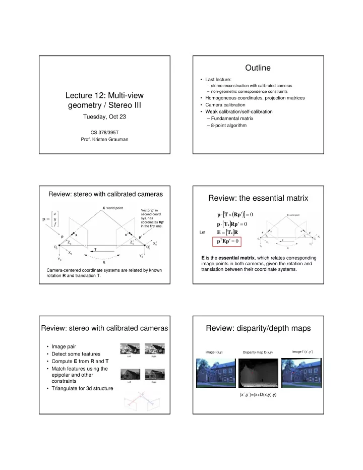Review: stereo with calibrated cameras Review: disparity/depth maps • Image pair image I´(x´,y´) image I(x,y) Disparity map D(x,y) • Detect some features • Compute E from R and T • Match features using the epipolar and other constraints • Triangulate for 3d structure (x´,y´)=(x+D(x,y),y)

Review: correspondence problem Review: correspondence problem • To find matches in the image pair, assume – Most scene points visible from both views Multiple – Image regions for the matches are similar in match appearance hypotheses • Dense or sparse matches satisfy • Additional (non-epipolar) constraints: epipolar – Similarity constraint, – Uniqueness but which is – Ordering correct? – Figural continuity – Disparity gradient Figure from Gee & Cipolla 1999 Homogeneous coordinates Review: correspondence error sources • Low-contrast / textureless image regions • Extend Euclidean space: add an extra coordinate • Points are represented by equivalence classes • Occlusions • Why? This will allow us to write process of • Camera calibration errors perspective projection as a matrix • Poor image resolution • Violations of brightness constancy (specular 2d: (x, y)’ � (x, y, 1)’ Mapping to reflections) homogeneous 3d: (x, y, z)’ � (x, y, z, 1)’ coordinates • Large motions 2d: (x, y, w)’ � (x/w, y/w)’ Mapping back from homogeneous 3d: (x, y, z, w)’ � (x/w, y/w, z/w)’ coordinates Homogeneous coordinates Perspective projection equations •Equivalence relation: Image plane Focal length (x, y, z, w) is the same as (kx, ky, kz, kw) Optical Camera axis frame Homogeneous coordinates are only defined up to a scale Scene point Image coordinates

Projection matrix for perspective projection Projection matrix for perspective projection fY fX y = x = Z Z From pinhole From pinhole camera model camera model Same thing, but written in terms of homogeneous coordinates Camera parameters Projection matrix for orthographic projection • Extrinsic: location and orientation of camera frame with respect to reference frame • Intrinsic: how to map pixel coordinates to image plane coordinates 1 Reference frame X Y x = y = Camera 1 frame 1 1 Rigid transformations Rotation about coordinate axes in 3d Combinations of rotations and translation Express 3d rotation as • Translation: add values to coordinates series of rotations around coordinate • Rotation: matrix multiplication α β γ , , axes by angles Overall rotation is product of these elementary rotations: R = R R R x y z

Camera parameters Extrinsic camera parameters • Extrinsic: location and orientation of camera = − frame with respect to reference frame P R ( P T ) c w • Intrinsic: how to map pixel coordinates to image plane coordinates Point in camera Point in world reference frame ( ) = Reference P X , Y , Z frame c Camera 1 frame Intrinsic camera parameters Camera parameters • We know that in terms of camera reference frame: • Ignoring any geometric distortions from optics, we can describe them by: = − − x ( x o ) s • Substituting previous eqns describing intrinsic and im x x extrinsic parameters, can relate pixels coordinates = − − to world points: y ( y o ) s Τ − im y y R ( P T ) − − = 1 w ( x o ) s f Τ im x x − ( ) R P T R i = Row i of 3 w rotation matrix Τ − Coordinates of Coordinates of Coordinates of Effective size of a R ( P T ) − − = 2 projected point in image point in image center in pixel (mm) w ( y o ) s f Τ im y y − camera reference pixel units pixel units R ( P T ) frame 3 w Linear version of perspective Calibrating a camera projection equations point in camera coordinates • Compute intrinsic and extrinsic • This can be rewritten X w x 1 parameters using observed as a matrix product = M int M ext Y w x 2 camera data using homogeneous Z w x 3 coordinates: 1 Main idea = x x / x im 1 3 • Place “calibration object” with = y x / x im 2 3 known geometry in the scene • Get correspondences Τ − r r r R T − 11 12 13 1 f / s 0 o • Solve for mapping from scene Τ x x − M int = − r r r R T 0 f / s o M ext = 21 22 23 2 to image: estimate M = M int M ext y y Τ − 0 0 1 r r r R T 31 32 33 3

Linear version of perspective Estimating the projection matrix projection equations P w in homog. ⋅ M P = − ⋅ • This can be rewritten X w = x 1 1 w 0 ( M x M ) P x ⋅ as a matrix product im 1 im 3 w = M int M ext Y w M P x 2 3 w using homogeneous Z w x 3 ⋅ M P coordinates: = M 1 = − ⋅ 2 w y 0 ( M y M ) P im ⋅ M P 2 im 3 w 3 w product M is single ⋅ M P = projection matrix = 1 w x x x / x encoding both im ⋅ M P im 1 3 extrinsic and intrinsic 3 w = ⋅ parameters y M x P / x = y 2 w im 2 3 ⋅ Let M i be row im M P 3 w i of matrix M Estimating the projection matrix Estimating the projection matrix = − ⋅ 0 ( M x M ) P 1 im 3 w Τ Τ Τ − = − ⋅ 0 ( M y M ) P M P 0 x P For a given feature point: 2 im 3 w 1 0 w im w = M Τ Τ − T 2 0 0 P y P = − ⋅ M 0 ( M x M ) P w im w 3 1 im 3 w = − ⋅ 0 ( M y M ) P 2 im 3 w Expanding this to see the elements: In matrix form: − − − − 0 = X Y Z 1 0 0 0 0 x X x Y x Z x w w w im w im w im w im Τ Τ Τ − − − − − 0 0 0 0 0 X Y Z 1 y X y Y y Z y P 0 x P M w w w im w im w im w im 1 0 = w im w M Τ Τ − T 2 0 0 P y P M w im w 3 Stack rows of matrix M Estimating the projection matrix Summary: camera calibration This is true for every feature point, so we can stack up n • Associate image points with scene points observed image features and their associated 3d points in single equation: Pm = 0 on object with known geometry P m • Use together with perspective projection − − − − ( 1 ) ( 1 ) ( 1 ) ( 1 ) ( 1 ) ( 1 ) ( 1 ) ( 1 ) ( 1 ) ( 1 ) X Y Z 1 0 0 0 0 x X x Y x Z x relationship to estimate projection matrix w w w im w im w im w im − − − − ( 1 ) ( 1 ) ( 1 ) ( 1 ) ( 1 ) ( 1 ) ( 1 ) ( 1 ) ( 1 ) ( 1 ) 0 0 0 0 X Y Z 1 y X y Y y Z y im w w w w im w im w im 0 = • (Can also solve for explicit parameters … … … … 0 − − − − ( n ) ( n ) ( n ) ( n ) ( n ) ( n ) ( n ) ( n ) ( n ) ( n ) X Y Z 1 0 0 0 0 x X x Y x Z x themselves) … w w w im w im w im w im − − − − ( n ) ( n ) ( n ) ( n ) ( n ) ( n ) ( n ) ( n ) ( n ) ( n ) 0 0 0 0 X Y Z 1 y X y Y y Z y 0 = im w w w w im w im w im 0 Solve for m ij ’s (the calibration information) with least squares. [F&P Section 3.1]