La rgression sous WinBugs: une vieille mthode revisite partir d'un - - PowerPoint PPT Presentation

1

JOURNEES Club WinBUGS 7 décembre 2006

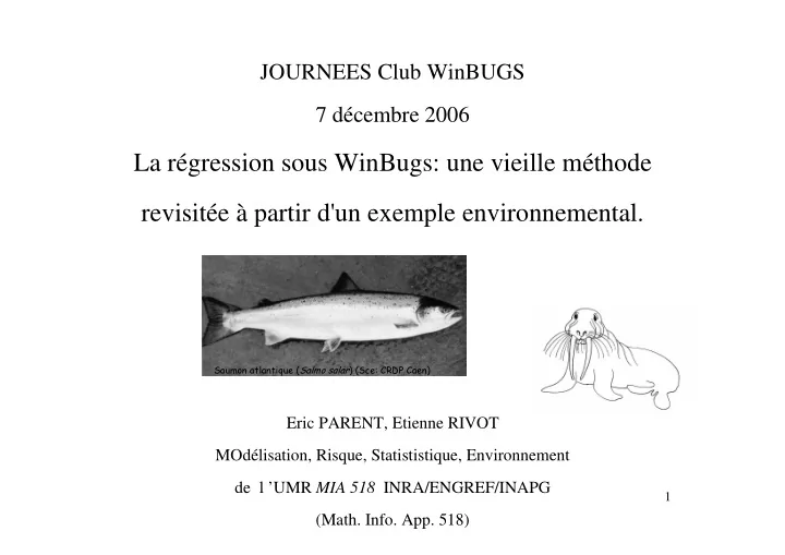
La régression sous WinBugs: une vieille méthode revisitée à partir d'un exemple environnemental.

Eric PARENT, Etienne RIVOT MOdélisation, Risque, Statististique, Environnement de l’UMR MIA 518 INRA/ENGREF/INAPG (Math. Info. App. 518)

Basics for regression

• Population vs sample
• True parameters vs estimates
• Hypotheses

Représentation graphique des notions suivantes : population (bleues), modèle (droite bleue), échantillon (croix rouges), modèle ajusté (droite rouge)

Représentation graphique de l'échantillon (croix rouges) et du modèle ajusté (droite rouge). La droite rouge obtenue est conditionnelle à l'échantillon en main (4 échantillons 4 droites différentes). Les coefficients (pente, ordonnée à l'origine et r2) sont donc incertains

Hypotheses

• Residuals are independant
• Residuals are from the same pdf
• Residuals are normal
• model structure

Distribution des résidus e

y y

i i i

= − en fonction de

• y

a bx

i i

= +

.

Normal PDF

( , ) ; X known Z µ µ σ σ − =

Bayes theory for the linear model

Remember Bayesian statistics ?

[ ] [ ] [ ]

[ ]

y y y θ × θ = θ

• Prior information

Posterior information DATA (y)

[ ]

θ

[ ]

y θ

Bayesian analysis of the linear model

t t t

x y ε β α + + = ) , ( ~

2

σ ε N

t

where

[ ]

( )( ) { }

      − − − ×       = θ θ σ σ π σ β α X Y X Y X y

n

’ 2 1 exp 2 1 , , ,

2 2

      − − − −       ∝      

∑

− − 1 2 1 2 2

) ( )’ ( 2 1 exp exp 1 1 , θ θ θ θ σ σ σ θ b H

a

β α θ = = = ; ... ... 1 ... ... 1 1 ; ... ...

1 1 n t n t

x x x X y y y Y

1/σ2~Gamma(a,b)

) , ( ~

0 Σ

θ θ N

Bayesian analysis of the linear model

ε θ + = X Y ) , ( ~

2I

N σ ε

where

[ ]

( )( ) { }

      + − − + − − − ×       = ) ˆ ˆ ( ' ˆ ˆ ( 2 1 exp 2 1 , , ,

2 2

θ θ θ θ θ θ σ σ π σ β α X Y X Y X y

n

2 1 2 1 2

exp 1 ) ( )’ ( 2 1 exp 1 , σ σ θ θ θ θ σ θ b H

a

−             − − − ∝      

− −

∑

( )

Y X X X ’ ’ ˆ

1 −

= θ

[ ]

( )(

)(

) ( )( ) { }

      − − + − − − ∝ θ θ θ θ θ θ σ σ β α ˆ ' ˆ ˆ ' ' ˆ 2 1 exp , , ,

2 2

X Y X Y X X X y

Least square estimate Pythagore’ theorem θ only!

Bayesian analysis of the linear model

ε θ + = X Y ) , ( ~

2I

N σ ε

where

( ) ( )

       −       − + − − − ∝      

∑

−1 2 2

ˆ ' ' ˆ ) ( )' ( 2 1 exp , , 1 θ θ σ θ θ θ θ θ θ θ σ X X X Y

( )

Y X X X ’ ’ ˆ

1 −

= θ

Least square estimate

) , ( ~

1 1 2

Σ θ σ θ N

If σ were known, θ would be normal

θ σ θ θ σ ˆ ' '

1 2 1 1 1 1 2 1 1

∑ ∑ ∑ ∑

− − − −

      + =       + = X X X X

Addition of the precision matrices Linear combination between prior mean and least square estimates

Bayesian analysis of the linear model

ε θ + = X Y ) , ( ~

2I

N σ ε

where

Gamma (a,b)

) ’ , ’ ( ~ 1

2

b a gamma θ σ

If θ were known, σ2 would be inverse Gamma(a’,b’)

2 ) ( )’ ( ’ 2 ’ θ θ X Y X Y b b n a a − − + = + =

( )

) ( )’ ( 2 1 exp 2 1 exp 1 , , 1

2 2 2 2 1 2 2

θ θ σ πσ σ σ θ σ X Y X Y b X Y

n a

− − −       −       ∝      

−

Stock Recruitment issues

• Fishing should not endanger population

conservation

• How many spawners are necessary to guarantee

salmon population conservation ?

• How does the number of spawners influence on

the recruitment ?

• Models of stock/recruitment relationship wanted

Margaree River

Margaree River

SALMON: The Salmon fishing season begins June 1 and ends October 31 ( fly

• nly ).Resident fees are set at $36.06. Non-

resident anglers must pay $133.19 for a seasonal license or $54.26 for a 7 day

• license. Bag limit: 2 per day and 8 per

season ( only grilse up to 63 cm 24.8 inches )

Margaree River

MARGAREE River

1000 2000 3000 4000 5000 6000 7000 8000 1000 2000 3000 4000 5000 6000 Géniteurs Recrues

Cohorte Géniteurs Recrues 1947 1685 4852 1948 3358 7204 1949 1839 5716 1950 1744 4000 1951 2093 2440 1952 969 2833 1956 486 2616 1957 822 4534 1961 344 3620 1962 1306 3850 1963 887 3538 1964 1053 2515 1965 993 3694 1966 727 1393 1967 1009 2083 1968 828 2378 1969 488 3394 1970 901 2702 1971 351 2630 1972 373 3261 1973 393 3131 1974 436 1066 1975 293 2813 1976 366 1819 1977 538 2909 1978 699 3292 1979 363 1868 1980 681 1462 1981 618 3616 1982 760 4015 1983 657 1688 1984 381 2289 1985 1378 5156 1986 3461 3484 1987 3899 6375 1988 1545 3358 1989 2164 2900 1990 5022 2365

A look at the data of SR Margaree river

1000 2000 3000 4000 5000 6000 7000 8000 1000 2000 3000 4000 5000 6000

Stock (nb reproducteurs) Recrutement (nb retours adultes)

Pick your own model!

• R as a function of S :

– a smooth idealized phenomenon R= µR(S), – when S ↑, R ↑ (at least at the beginning)

⇒ R est fonction de S

• Indeed R is uncertain for many reasons (S is the only explanation available)

⇒ stochastic model

• Math. translation :

R ~ pdf with caracteristics (µR(S), σ)

– position parameter µR(S), dispersion parameter σ – dispersion parameter σ is not a fonction of S

• µR(S) ? Which pdf ?

Searching for a model

Searching for µR(S)

• µR(S) ?

– Ecological knowledge : competition for territory – R ↑ then S ↑, then R stops or decreases

⇒ Feedback control by density

• 2 classical functions :

– Beverton-Holt µR(S) = aS/(1 + bS) reproduction ratio µR(S)/S = a/(1 + bS) – Ricker µR(S) = aSe-bS

reproduction rate µR(S)/S = ae-bS

– Log(µR(S)/S)=Log(a)-bS

Fonctions Ricker et BH

0,5 1 1,5 2 2,5 3 3,5 50 100 150 200

S

muR(S)/S

BH Ricker

10 20 30 40 50 60 50 100 150 200

S

muR(S)

BH Ricker

Beverton-Holt µR(S)/S = a/(1 + bS) Ricker µR(S)/S = ae-bS

Ricker = a hidden linear model

• Summing up

– R ~ logN(µR(S), σ) – µR(S) = aSe-bS (Ricker function) – deterministic explanatory structure + random effect

• bS

R R

aSe S N e S R

−

= = ) ( ) , ( ~ ) (

2

µ σ ε µ

ε

) ), (log( ) log( log ) log( ) log( ) log( b a b a S x S R y bS S a R = − = = =       = + − + = θ β α ε

) , ( ~

2

σ ε ε β α N x y + + =

DAG of the Ricker SR model: classical formulation

st ß ~ unif a ~ unif Ricker function : R(st) = stexp(a - ßst) t = 1 to T observations rt,~ LogN(µRt, σ) σ ~ uninf

log(σ 2) ~ unif

µRt = log(R(st))

DAG of the Ricker SR model: classical formulation

st ß ~ unif a ~ unif Ricker function : R(st) = stexp(a - ßst) t = 1 to T observations rt,~ LogN(µRt, σ) σ ~ uninf

log(σ 2) ~ unif

µRt = log(R(st)) Slope = exp(a) Smax = 1/ß

Posterior inference….

model fit: r.star 0.0 2.0E+3 4.0E+3 6.0E+3

r.star 0.0 5.0E+3 1.0E+4 1.5E+4

tau 0.05.0 10.0 15.0

alpha sample: 30001 alpha 1.25 1.5 1.75 2.0 2.25 2.5

P(alpha) 0.0 2.0 4.0

beta sample: 30001 beta 2.0E-4 4.0E-4 6.0E-4

P(beta) 0.0 6.0E+3 tau sample: 30001 tau 0.0 5.0 10.0 P(tau) 0.0 0.2 0.4

2 4 6 8 10 12 5 10 15

• eufs déposés/m²
• eufs

recrutés/m²

production remplacement excédent

Reference points of the Ricker function

SMSY MSY

CHANGE of PARAMETERS Schnute & Kronlund formulation

st Sopt ~ ? Copt ~ ? Ricker function : R(st) = stexp(a - ßst) t = 1 to T observations rt,~ LogN(µRt, σ) σ ~ uninf

log(σ 2) ~ unif

µRt = log(R(st)) a

= log((Copt + Sopt)/Sopt) + (Copt/(Sopt + Copt))

ß

= Copt/(Sopt(Sopt + Copt))

Which priors to assign to Copt and Sopt?

• Option 0 : uniformative priors to and
• Option 1: assign a prior equivalent to the reference

prior assigned to and

• Option 2: propose a little informative prior(s) based
• n some rationale

Posterior Analysis 2

model fit: r.star 0.0 2.0E+3 4.0E+3

r.star 0.0 5.0E+3 1.5E+4

alpha sample: 20001 alpha 1.25 1.5 1.75 2.0 2.25 2.5

P(alpha) 0.0 2.0 4.0

beta sample: 20001 beta 0.0 2.0E-4 6.0E-4

P(beta) 0.0 6.0E+3

tau sample: 20001 tau 0.0 5.0 10.0

P(tau) 0.0 0.2

Copt sample: 30000 Copt 0.0 2.0E+3 4.0E+3

P(Copt) 0.0 0.001

Sopt sample: 30000 Sopt 0.0 1.0E+3 3.0E+3

P(Sopt) 0.0 0.002

5% 50% 95% Copt 2378.0 2926.0 3636.0 Sopt 1170.0 1425.0 1881.0

Caution is required when changing parameterization (Rivot et al., 2001): it may carry additional (implicit) hypothesis

• in the case of the Ricker model: the management related

parameterization assumes at least a segment of the Ricker curve is above replacement ⇔ ⇔ slope > 1

• this is a very strong a prior hypothesis for weak population

hardly able to replace generations

• Recommendations:
• always start with classical parameters and priors not
• assess sensitivity of results to various reasonable

priors/parametrization

Under the standard lognormal formulation, recruitment variance is proportional to the square of the Ricker function ⇒ for s > Smax, recruitment variance decreases with s Alternative hypothesis: recruitment variance is proportional to s Implementation is easy with assuming a gamma distribution for the recruitment (not possible with lognormal)

• X ~ gamma(a, b), a = shape, b = inverse scale
• E(X) = a/b
• Var(X) = a/b2 = E(X)/b
• Given the above, propose a formulation for which mean

recruitment is the Ricker function and recruitment variance is proportional to the stock

CHANGE OF ERROR

Ricker model DAG : (variance ∝ stock) formulation

st Sopt ~ ? Copt ~ ? Ricker function : R(st) = stexp(a - ßst) t = 1 to T observations rt,~ Gamma(at,bt) d ~ uninf

log(d) ~ unif

at a

= log((Copt + Sopt)/Sopt) + (Copt/(Sopt + Copt))

ß

= Copt/(Sopt(Sopt + Copt))

bt

Ricker with gamma errors

model fit: r.star 0.0 2.0E+3 4.0E+3

r.star 0.0 5.0E+3 1.0E+4

Sopt sample: 10001 Sopt 500.0 1.0E+3 1500.0 2.0E+3

P(Sopt) 0.0 0.002

5% 50% 95% Copt 2379.0 2805.0 3334.0 Sopt 1070.0 1411.0 1870.0

Copt sample: 10001 Copt 2.0E+3 3.0E+3 4.0E+3

P(Copt) 0.0 0.001

CHANGE OF MODEL Beverton&Holtz =a non linear model

• Summing up

– R ~ logN(µR(S), σ) – µR(S) = aS/(1 + bS) (Beverton & Holtz type ) – deterministic explanatory structure + random effect

• bS

aS S N e S R

R R

+ = = 1 ) ( ) , ( ~ ) (

2

µ σ ε µ

ε

) ), (log( ) log( log ) 1 log( ) log( ) log( ) log( b a b a S x S R y bS S a R = = = =       = + + − + = θ β α ε

) , ( ~ ) 1 log(

2

σ ε ε β α N x y + + − =

Inference of RS relationships

• Ricker : use the standart linear model theory

If bayesian, what becomes the prior knowledge (if any) after reparametrization?

• Beverton-Holtz : use non linear techniques

If bayesian, which prior [θ,σ]? Then MCMC…(see WinBugs in a while)

[ ]

( )

∏

=

        + − − − =

T t t T t

x y y y y

1 2 2 1

) 1 log( 2 1 exp 2 1 , ,... ,.. β α σ σ π σ θ

To sum it up...

Modèle Ricker classique Schnute/Kronlund a 6,02558 1381 Sopt b 0,00049 2859 Copt SCE 6,17671 6 Beverton/Holt classique Schnute/Kronlund a 13,58068 835 Sopt b 0,00321 2243 Copt SCE 5,10412 5

Summary

• R-S curves : Bayes inference at work

Ricker a hidden linear model….

• Reparametrisation : statistical natural

parameters are seldom meaningful for practitionners -> prior modelling

• Role of the error term : what is ε ?
• Discuss the hypotheses

– Change R/S structure – S not known, only observed

Conclusion Our inferences are not sensitive to priors: the data set is long and informative (good contrast in the spawning stock level) But Inferences are more sensitive to modelling hypotheses (recruitment variance proportional to stock or to recruitment) Which model is best? Model choice by calculating posterior odds of competing models

References

• Millar R.B., 2002. Reference priors for Bayesian fisheries
• models. Can. J. Fish. Aquat. Sci., 59: 1492-1502

Rivot E., Prévost E., Parent E., 2001. How robust are Bayesian posterior inferences based on a Ricker model with regards to measurement errors and prior assumptions about parameters? Can. J. Fish. Aquat. Sci., 58: 2284-2297. Schnute, J. T., and Kronlund, A. R. 1996. A management

• riented approach to stock recruitment analysis. Canadian

Journal of Fisheries and Aquatic Sciences, 53: 1281-1293

Bernier, J., Parent, E. et J-J Boreux (2000), Statistique pour l’environnement : traitement bayésien de l'incertitude, Eds Tec & Doc (Lavoisier), Paris (363 p.).

• Texte «pédagogique»
• Mathématiques

– Niveau «bac» – + quatre intégrales

• Prix : 65