Presentation 7.3a: Multiple linear re- gression Murray Logan July - - PDF document

• 1-

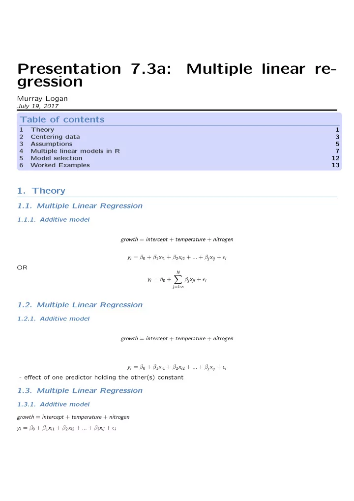
Presentation 7.3a: Multiple linear re- gression

Murray Logan

July 19, 2017

Table of contents

1 Theory 1 2 Centering data 3 3 Assumptions 5 4 Multiple linear models in R 7 5 Model selection 12 6 Worked Examples 13

• 1. Theory

1.1. Multiple Linear Regression

1.1.1. Additive model growth = intercept + temperature + nitrogen yi = β0 + β1xi1 + β2xi2 + ... + βjxij + ϵi OR yi = β0 +

N

∑

j=1:n

βjxji + ϵi

1.2. Multiple Linear Regression

1.2.1. Additive model growth = intercept + temperature + nitrogen yi = β0 + β1xi1 + β2xi2 + ... + βjxij + ϵi

• effect of one predictor holding the other(s) constant

1.3. Multiple Linear Regression

1.3.1. Additive model growth = intercept + temperature + nitrogen yi = β0 + β1xi1 + β2xi2 + ... + βjxij + ϵi

• 2-

Y X1 X2 3 22.7 0.9 2.5 23.7 0.5 6 25.7 0.6 5.5 29.1 0.7 9 22 0.8 8.6 29 1.3 12 29.4 1

1.4. Multiple Linear Regression

1.4.1. Additive model 3 = β0 + (β1 × 22.7) + (β2 × 0.9) + ε1 2.5 = β0 + (β1 × 23.7) + (β2 × 0.5) + ε2 6 = β0 + (β1 × 25.7) + (β2 × 0.6) + ε3 5.5 = β0 + (β1 × 29.1) + (β2 × 0.7) + ε4 9 = β0 + (β1 × 22) + (β2 × 0.8) + ε5 8.6 = β0 + (β1 × 29) + (β2 × 1.3) + ε6 12 = β0 + (β1 × 29.4) + (β2 × 1) + ε7

1.5. Multiple Linear Regression

1.5.1. Multiplicative model growth = intercept + temp + nitro + temp × nitro yi = β0 + β1xi1 + β2xi2 + β3xi1xi2 + ... + ϵi

1.6. Multiple Linear Regression

1.6.1. Multiplicative model

3 = β0 + (β1 × 22.7) + (β2 × 0.9) + (β3 × 22.7 × 0.9) + ε1 2.5 = β0 + (β1 × 23.7) + (β2 × 0.5) + (β3 × 23.7 × 0.5) + ε2 6 = β0 + (β1 × 25.7) + (β2 × 0.6) + (β3 × 25.7 × 0.6) + ε3 5.5 = β0 + (β1 × 29.1) + (β2 × 0.7) + (β3 × 29.1 × 0.7) + ε4 9 = β0 + (β1 × 22) + (β2 × 0.8) + (β3 × 22 × 0.8) + ε5 8.6 = β0 + (β1 × 29) + (β2 × 1.3) + (β3 × 29 × 1.3) + ε6 12 = β0 + (β1 × 29.4) + (β2 × 1) + (β3 × 29.4 × 1) + ε7

• 3-
• 2. Centering data

2.1. Multiple Linear Regression

2.1.1. Centering

• ●
• ●
• 10

20 30 40 50 60

x

−20 −10 10 20

y

2.2. Multiple Linear Regression

2.2.1. Centering

• 47

48 49 50 51 52 53 54

2.3. Multiple Linear Regression

• 4-

2.3.1. Centering

• 47

48 49 50 51 52 53 54

2.4. Multiple Linear Regression

2.4.1. Centering

• 47

48 49 50 51 52 53 54 −3 −2 −1 1 2 3 4

• 5-

2.5. Multiple Linear Regression

2.5.1. Centering

• −4

−2 2 4

cx1

16 18 20 22 24

y

• 3. Assumptions

3.1. Multiple Linear Regression

3.1.1. Assumptions Normality, homog., linearity

3.2. Multiple Linear Regression

3.2.1. Assumptions (multi)collinearity

• 6-

3.3. Multiple Linear Regression

3.3.1. Variance inflation Strength of a relationship R2 Strong when R2 ≥ 0.8

3.4. Multiple Linear Regression

3.4.1. Variance inflation var.inf = 1 1 − R2 Collinear when var.inf >= 5 Some prefer > 3

3.5. Multiple Linear Regression

3.5.1. Assumptions (multi)collinearity

library(car) # additive model - scaled predictors vif(lm(y ~ cx1 + cx2, data))

cx1 cx2 1.743817 1.743817

3.6. Multiple Linear Regression

3.6.1. Assumptions (multi)collinearity

library(car) # additive model - scaled predictors vif(lm(y ~ cx1 + cx2, data))

• 7-

cx1 cx2 1.743817 1.743817

# multiplicative model - raw predictors vif(lm(y ~ x1 * x2, data))

x1 x2 x1:x2 7.259729 5.913254 16.949468

3.7. Multiple Linear Regression

3.7.1. Assumptions

# multiplicative model - raw predictors vif(lm(y ~ x1 * x2, data))

x1 x2 x1:x2 7.259729 5.913254 16.949468

# multiplicative model - scaled predictors vif(lm(y ~ cx1 * cx2, data))

cx1 cx2 cx1:cx2 1.769411 1.771994 1.018694

• 4. Multiple linear models in R

4.1. Model fitting

Additive model yi = β0 + β1xi1 + β2xi2 + ϵi

data.add.lm <- lm(y~cx1+cx2, data)

4.2. Model fitting

Additive model yi = β0 + β1xi1 + β2xi2 + ϵi

data.add.lm <- lm(y~cx1+cx2, data)

Multiplicative model yi = β0 + β1xi1 + β2xi2 + β3xi1xi2 + ϵi

data.mult.lm <- lm(y~cx1+cx2+cx1:cx2, data) #OR data.mult.lm <- lm(y~cx1*cx2, data)

4.3. Model evaluation

Additive model

plot(data.add.lm)

• 8-

−3 −2 −1 −2 −1 1 2 Fitted values Residuals

• ●
• Residuals vs Fitted

30 40 74

• −2

−1 1 2 −2 −1 1 2 Theoretical Quantiles Standardized residuals

Normal Q−Q

40 30 74

−3 −2 −1 0.0 0.5 1.0 1.5 Fitted values Standardized residuals

• Scale−Location

40 30 74

0.00 0.02 0.04 0.06 −2 −1 1 2 Leverage Standardized residuals

• Cook's distance

Residuals vs Leverage

40 19 10

4.4. Model evaluation

Multiplicative model

plot(data.mult.lm)

−4 −3 −2 −1 1 2 −2 −1 1 2 Fitted values Residuals

• ●
• Residuals vs Fitted

30 74 59

• ●
• −2

−1 1 2 −2 −1 1 2 Theoretical Quantiles Standardized residuals

Normal Q−Q

30 7459

−4 −3 −2 −1 1 2 0.0 0.5 1.0 1.5 Fitted values Standardized residuals

• Scale−Location

30 74 59

0.00 0.05 0.10 0.15 0.20 −2 −1 1 2 Leverage Standardized residuals

• ●
• Cook's distance

Residuals vs Leverage

40 84 19

• 9-

4.5. Model summary

Additive model

summary(data.add.lm)

Call: lm(formula = y ~ cx1 + cx2, data = data) Residuals: Min 1Q Median 3Q Max

• 2.39418 -0.75888 -0.02463

0.73688 2.37938 Coefficients: Estimate Std. Error t value Pr(>|t|) (Intercept)

• 1.5161

0.1055 -14.364 < 2e-16 *** cx1 2.5749 0.4683 5.499 3.1e-07 *** cx2

• 4.0475

0.3734 -10.839 < 2e-16 ***

• Signif. codes:

0 '***' 0.001 '**' 0.01 '*' 0.05 '.' 0.1 ' ' 1 Residual standard error: 1.055 on 97 degrees of freedom Multiple R-squared: 0.5567, Adjusted R-squared: 0.5476 F-statistic: 60.91 on 2 and 97 DF, p-value: < 2.2e-16

4.6. Model summary

Additive model

confint(data.add.lm)

2.5 % 97.5 % (Intercept) -1.725529 -1.306576 cx1 1.645477 3.504300 cx2

• 4.788628 -3.306308

4.7. Model summary

Multiplicative model

summary(data.mult.lm)

Call: lm(formula = y ~ cx1 * cx2, data = data) Residuals: Min 1Q Median 3Q Max

• 2.23364 -0.62188

0.01763 0.80912 1.98568 Coefficients: Estimate Std. Error t value Pr(>|t|) (Intercept)

• 1.6995

0.1228 -13.836 < 2e-16 *** cx1 2.7232 0.4571 5.957 4.22e-08 *** cx2

• 4.1716

0.3648 -11.435 < 2e-16 ***

• 10-

cx1:cx2 2.5283 0.9373 2.697 0.00826 **

• Signif. codes:

0 '***' 0.001 '**' 0.01 '*' 0.05 '.' 0.1 ' ' 1 Residual standard error: 1.023 on 96 degrees of freedom Multiple R-squared: 0.588, Adjusted R-squared: 0.5751 F-statistic: 45.66 on 3 and 96 DF, p-value: < 2.2e-16

4.8. Graphical summaries

Additive model

library(effects) plot(effect("cx1",data.add.lm, partial.residuals=TRUE))

cx1 effect plot

cx1 y

−4 −3 −2 −1 1 2 3 −0.4 −0.2 0.0 0.2 0.4

• 4.9. Graphical summaries

Additive model

library(effects) library(ggplot2) e <- effect("cx1",data.add.lm, xlevels=list( cx1=seq(-0.4,0.4, len=10)), partial.residuals=TRUE) newdata <- data.frame(fit=e$fit, cx1=e$x, lower=e$lower, upper=e$upper) resids <- data.frame(resid=e$partial.residuals.raw, cx1=e$data$cx1)

Error in data.frame(resid = e$partial.residuals.raw, cx1 = e$data$cx1): arguments imply differing number of rows: 0, 100

ggplot(newdata, aes(y=fit, x=cx1)) + geom_point(data=resids, aes(y=resid, x=cx1))+ geom_ribbon(aes(ymin=lower, ymax=upper), fill='blue', alpha=0.2)+ geom_line()+theme_classic()

Error in fortify(data): object 'resids' not found

• 11-

4.10. Graphical summaries

Additive model

library(effects) plot(allEffects(data.add.lm))

cx1 effect plot

cx1 y

−3.0 −2.5 −2.0 −1.5 −1.0 −0.5 0.0 −0.4 −0.2 0.0 0.2 0.4

cx2 effect plot

cx2 y

−4 −3 −2 −1 1 −0.4 −0.2 0.0 0.2 0.4

4.11. Graphical summaries

Multiplicative model

library(effects) plot(allEffects(data.mult.lm))

cx1*cx2 effect plot

cx1 y

−6 −4 −2 −0.4 −0.2 0.0 0.2 0.4

= cx2 −0.5

−0.4 −0.2 0.0 0.2 0.4

= cx2

−0.4 −0.2 0.0 0.2 0.4

= cx2 0.5

4.12. Graphical summaries

Multiplicative model

library(effects) plot(Effect(focal.predictors=c("cx1","cx2"),data.mult.lm))

• 12-

cx1*cx2 effect plot

cx1 y

−6 −4 −2 −0.4 −0.2 0.0 0.2 0.4

= cx2 −0.5

−0.4 −0.2 0.0 0.2 0.4

= cx2

−0.4 −0.2 0.0 0.2 0.4

= cx2 0.5

• 5. Model selection

5.1. How good is a model?

“All models are wrong, but some are useful” George E. P. Box 5.1.1. Criteria

• R2 - no
• Information criteria

– AIC, AICc – penalize for complexity

5.2. Model selection

5.2.1. Candidates

AIC(data.add.lm, data.mult.lm)

df AIC data.add.lm 4 299.5340 data.mult.lm 5 294.2283

library(MuMIn) AICc(data.add.lm, data.mult.lm)

df AICc data.add.lm 4 299.9551 data.mult.lm 5 294.8666

5.3. Model selection

5.3.1. Dredging

library(MuMIn) data.mult.lm <- lm(y~cx1*cx2, data, na.action=na.fail) dredge(data.mult.lm, rank="AICc", trace=TRUE)

• 13-

0 : lm(formula = y ~ 1, data = data, na.action = na.fail) 1 : lm(formula = y ~ cx1 + 1, data = data, na.action = na.fail) 2 : lm(formula = y ~ cx2 + 1, data = data, na.action = na.fail) 3 : lm(formula = y ~ cx1 + cx2 + 1, data = data, na.action = na.fail) 7 : lm(formula = y ~ cx1 + cx2 + cx1:cx2 + 1, data = data, na.action = na.fail) Global model call: lm(formula = y ~ cx1 * cx2, data = data, na.action = na.fail)

• Model selection table

(Int) cx1 cx2 cx1:cx2 df logLik AICc delta weight 8 -1.699 2.7230 -4.172 2.528 5 -142.114 294.9 0.00 0.927 4 -1.516 2.5750 -4.047 4 -145.767 300.0 5.09 0.073 3 -1.516

• 2.706

3 -159.333 324.9 30.05 0.000 1 -1.516 2 -186.446 377.0 82.15 0.000 2 -1.516 -0.7399 3 -185.441 377.1 82.27 0.000 Models ranked by AICc(x)

5.4. Multiple Linear Regression

5.4.1. Model averaging

library(MuMIn) data.dredge<-dredge(data.mult.lm, rank="AICc") model.avg(data.dredge, subset=delta<20)

Call: model.avg(object = data.dredge, subset = delta < 20) Component models: '123' '12' Coefficients: (Intercept) cx1 cx2 cx1:cx2 full

• 1.686125 2.712397 -4.162525 2.344227

subset

• 1.686125 2.712397 -4.162525 2.528328

5.5. Multiple Linear Regression

5.5.1. Model selection Or more preferable:

• identify 10-15 candidate models
• compare these via AIC (etc)
• 6. Worked Examples

6.1. Worked examples

loyn <- read.csv('../data/loyn.csv', strip.white=T) head(loyn)

• 14-

ABUND AREA YR.ISOL DIST LDIST GRAZE ALT 1 5.3 0.1 1968 39 39 2 160 2 2.0 0.5 1920 234 234 5 60 3 1.5 0.5 1900 104 311 5 140 4 17.1 1.0 1966 66 66 3 160 5 13.8 1.0 1918 246 246 5 140 6 14.1 1.0 1965 234 285 3 130

6.2. Worked Examples

Question: what effects do fragmentation variables have on the abundance of forest birds Linear model: Abundi = β0 +

N

∑

j=1:n

βjXji + εi ε ∼ N(0, σ2)