L. Li (LMD/CNRS): Atmospheric equations page 1 Derivative of a - - PowerPoint PPT Presentation

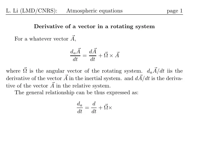
• L. Li (LMD/CNRS):

Atmospheric equations page 1 Derivative of a vector in a rotating system For a whatever vector A, da A dt = d A dt + Ω × A where Ω is the angular vector of the rotating system. da A/dt iis the derivative of the vector A in the inertial system. and d A/dt is the deriva- tive of the vector A in the relative system. The general relationship can be thus expressed as: da dt = d dt + Ω×

• L. Li (LMD/CNRS):

Atmospheric equations page 2 Expression of the acceleration term in rotating coordinates By applying the general relationship to the position vector r (defined as a vector from the Earth’s centre to the considered point at the Earth’s surface), we obtain the equation relating the absolute velocity and the relative velocity: da r dt = d r dt + Ω × r That is:

• Va =

V + Ω × r where Ω × r is the associated velocity due to the rotation of the Earth. The general derivative operator can be applied to the velocity vector itself Va: da Va dt = d Va dt + Ω × Va

• L. Li (LMD/CNRS):

Atmospheric equations page 3 This gives: da Va dt = d dt( V + Ω × r) + Ω × ( V + Ω × r) = d V dt + 2 Ω × V + Ω × ( Ω × r) = d V dt + 2 Ω × V − Ω2 R where R is a vector perpendicular to the axis of rotation, with magnitude equal to the distance to the axis of rotation. The absolute acceleration da Va/dt can thus be decomposed into three terms:

• relative acceleration d

V /dt,

• Coriolis acceleration 2

Ω × V and

• centripetal acceleration −Ω2

R.

• L. Li (LMD/CNRS):

Atmospheric equations page 4 Equations governing the atmosphere

• Equation of motion, momentum conservation
• Continuity equation, mass conservation
• Thermodynamic energy equation, energy conservation
• Equation of state for an ideal gas

• L. Li (LMD/CNRS):

Atmospheric equations page 5 Equation of motion For a particle of air of unit mass with ρ as the density, different forces can be identified, either ”real” or ”apparent”.

• The pressure gradient force

F = −1 ρ∇p.

• The viscous force

N = ν∇2 V where ν is the viscosity coefficient.

• The gravitational force

g = − GM

r3

r where G is the gravitational constant.

• The centrifugal force Ω2

R

• The Coriolis force −2

Ω × V

• The gravity force

g = − GM

r3

r + Ω2 R = −∇Φ. In practice, | g| changes only about 1% at maximum around the constant m/s2. The angle between g and r is always smaller than 0.2◦.

• L. Li (LMD/CNRS):

Atmospheric equations page 6 The centrifugal force and the Coriolis force are apparent ones, due to the rotation of the Earth. We have now the dynamic equation of the atmosphere: d V dt = −1 ρ∇p − 2 Ω × V + g + N

• L. Li (LMD/CNRS):

Atmospheric equations page 7 Mass conservation equation Mass divergence form: ∂ρ ∂t + ∇ · (ρ V ) = 0 Or velocity divergence form: dρ dt + ρ∇ · V = 0 Equation of state The thermodynamic state of the atmosphere at any point is deter- mined by the values of pressure, temperature, and density (or specific volume) at that point. These field variables are related to each other by the equation of state for ideal gas. p = ρRT

• L. Li (LMD/CNRS):

Atmospheric equations page 8 Energy conservation equation If the heating rate of a particle of air is Q (J kg−1s−1), the internal energy has to change Cv dT

dt and the particle works through compression

• r expansion by p d

dt( 1 ρ). The enrgy conservation equation is thus:

Cv dT dt + p d dt(1 ρ) = Q By using the equation of state, we can obtain: p d dt(1/ρ) = RdT dt − 1 ρ dp dt The energy conservation equation can thus be expressed in another form: Cp dT dt − 1 ρ dp dt = Q where Cp = Cv + R is the specific heat at constant pressure.

• L. Li (LMD/CNRS):

Atmospheric equations page 9 Potential temperature For an ideal gas undergoing an adiabatic process (i.e., a reversible process in which no heat is exchanged with the surroundings, Q = 0) the energy conservation equation can be written in the form Cpd ln T − Rd ln p = 0 Integrating this expression from a state at pressure p and temperature T to a state in which the pressure is p0 and the temperature is θ, we

• btain after taking the antilogarithm

θ = T p0 p R/Cp This relationship is referred to as Poisson’s equation, and the tempera- ture θ thus defined is called the potential temperature.

• L. Li (LMD/CNRS):

Atmospheric equations page 10 The spherical coordinates The three primative directions over the Earth are the longitude λ, latitude φ and the radial distance r from the center of the Earth. In practice, the third direction uses z, the distance from the sea level. Sup- pose that the radius of the Earth (a) is constant, one can obtain r = a+z and dr = dz. By using u, v and w to represent the three components of the velocity vector, we can have: u = r cos φdλ dt v = rdφ dt w = dr dt

• L. Li (LMD/CNRS):

Atmospheric equations page 11 Equation of motion in spherical coordinates For purpose of theoretical analysis and numerical prediction, it is necessary to expand the vectorial equation of motion into its scalar com- ponents: du dt = uv tan φ r − uw r − 1 ρr cos φ ∂p ∂λ + fv − ˆ fw + Nλ dv dt = −u2 tan φ r − vw r − 1 ρr ∂p ∂φ − fu + Nφ dw dt = u2 + v2 r − 1 ρ ∂p ∂r − g + ˆ fu + Nz The terms proportional to 1/r are called the curvature terms, owing to the curvature of the earth. f = 2Ω sin φ is the Coriolis parameter and ˆ f = 2Ω cos φ. Considering r = a + z with a ≫ z, one can replace r by a and dr by dz in the above equations.

• L. Li (LMD/CNRS):

Atmospheric equations page 12 Scale analysis of the equations of motion For synoptic-scale circulations, one can have: du dt = uv tan φ a −uw a − 1 ρa cos φ ∂p ∂λ +fv − ˆ fw +Nλ 10−4 10−5 10−8 10−3 10−3 10−6 10−5 dv dt = −u2 tan φ a −vw a − 1 ρa ∂p ∂φ −fu +Nφ 10−4 10−5 10−8 10−3 10−3 10−5 dw dt = u2v2 a −1 ρ ∂p ∂z −g + ˆ fu +Nz 10−7 10−5 10 10 10−3 10−7

• L. Li (LMD/CNRS):

Atmospheric equations page 13 Hydrostatic Approximation: ∂p ∂z = −ρg Geostropic Approximation: the pressure gradient force is approxi- matively in equilibrium with the Coriolis force: fvg = 1 ρa cos φ ∂p ∂λ fug = − 1 ρa ∂p ∂φ Or in vector form:

• vg = 1

ρf

• k × ∇p

One can see that the geostrophic balance is a diagnostic expression that gives the approximative relationship between the pressure field and hor- izontal velocity in large-scale extratropical systems. The geostrophic approximation is verified when the wind acceleration is much smaller than the Coriolis force.

• L. Li (LMD/CNRS):

Atmospheric equations page 14 Thermal wind This is an important notion to understand the general circulation

• f the atmosphere.

The thermal wind ( VT ) is defined as the vertical variation of the geostrophic wind:

• VT = ∂

Vg ∂z = R f

• k × ∇T

A horizontal temperature gradient can thus induce a wind vector that is parallel to the iso-temperature lines.

• L. Li (LMD/CNRS):

Atmospheric equations page 15 Primitive Equation The geostrophic equation is a diagnostic relation, since it does contain any terms of temporal derivative. One needs to take other terms with smaller values to obtain a prognostic equation: du dt = fv − 1 ρa cos φ ∂p ∂λ + Nλ dv dt = −fu − 1 ρa ∂p ∂φ + Nφ For phenomena with a spatial extension comparable to the radius of the Earth, such as stationary planetary waves, the Hadley cell, one needs also to take into consideration the terms in relation with the curvature

• f the Earth.

du dt = uv a tan φ + fv − 1 ρa cos φ ∂p ∂λ + Nλ dv dt = u2 a tan φ − fu − 1 ρa ∂p ∂φ + Nφ

• L. Li (LMD/CNRS):

Atmospheric equations page 16 Vorticity and potential vorticity Vorticity is a vector field defined as the curl of 3-dimensional velocity field ∇ ×

• V3d. It is the microscopic measure of rotation in a fluid. The

absolute vorticity is the curl of the absolute velocity, while the relative vorticity is the curl of the relative velocity. Although the vorticity is a vector field, we are in general concerned only with its vertical component, since the motions are mainly horizontal for large-scale dynamics of the atmosphere: k·(∇× V3d), that is, ζ = ∇× V = ∂v/∂x−∂u/∂y. Vorticity equation can be deduced from equation of motion. The potential vorticity is defined as the projection of the vorticity vector ∇× V3d onto the direction indicated by the potential temperature gradient ∇θ: P = 1 ρ(∇θ) · (∇ × V3d). By using the equation of motion, the continuity equation and the ther- modynamical equation, one can deduce the equation governing the po- tential vorticity. For an adiabatic motion without friction, a particle of air conserves its potential vorticity.

• L. Li (LMD/CNRS):

Atmospheric equations page 17 Equation of vorticity In Cartesian coordinates: ∂ ∂y ∂u ∂t + u∂u ∂x + v ∂u ∂y + w∂u ∂z − fv = −1 ρ ∂p ∂x

• ∂

∂x ∂v ∂t + u∂v ∂x + v ∂v ∂y + w∂v ∂z + fu = −1 ρ ∂p ∂y

• One can thus obtain:

d dt(ζ+f) = −(ζ+f) ∂u ∂x + ∂v ∂y

• −

∂w ∂x ∂v ∂z − ∂w ∂y ∂u ∂z

• + 1

ρ2 ∂ρ ∂x ∂p ∂y − ∂ρ ∂y ∂p ∂x

• Three terms contribute to the rate of change for absolute vorticity: the

divergence term, the tilting or twisting term, and the solenoidal term. For synoptic-scale atmospheric circulation, the divergence term is dom- inant: a horizontal convergence generates vorticity and a horizontal di- vergence destroys vorticity.

• L. Li (LMD/CNRS):

Atmospheric equations page 18 Furthermore, if the motion is non-divergent, the absolute vorticity is conserved. d dt(ζ + f) = 0. That is (with ∂f/∂x = 0 and β = ∂f/∂y): ∂ ∂t + u ∂ ∂x + v ∂ ∂y

• ζ + βv = 0.

This equation, studied by C. G. Rossby at the end of 1930, also known as Rossby Equation, is very useful for meteorological phenomena. The first numerical weather prediction was realized by J. Charney and his group at the beginning of 1950 through the Rossby equation.