L. Li (LMD/CNRS): LMDZ: a GCM of the atm. page 1 Climate modelling: - - PowerPoint PPT Presentation

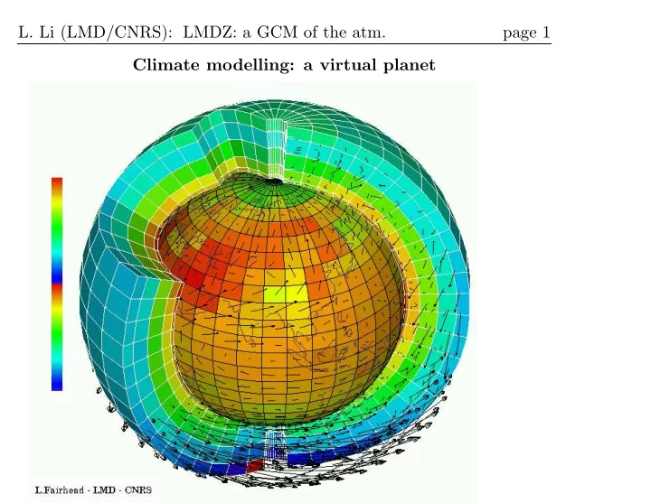
• L. Li (LMD/CNRS): LMDZ: a GCM of the atm.

page 1 Climate modelling: a virtual planet

• L. Li (LMD/CNRS): LMDZ: a GCM of the atm.

page 2 Physics in a GCM

processes Adiabatic winds temperature clouds humidity diffusion radiation condensation re−evaporation precipitation friction heat flux sensible evaporation roughness Ground temperature Ground Snow humidity Ground melting

• L. Li (LMD/CNRS): LMDZ: a GCM of the atm.

page 3 Numerical weather prediction, as imagined by J. Richardson

• L. Li (LMD/CNRS): LMDZ: a GCM of the atm.

page 4 Structure of LMDZ Requirements for running the GCM LMDZ: Availability of a For- tran compiler (G95 for example); Pre-installation of NetCDF library. Download the compressed “tar” file “gcm lmdz.tar.gz”. Retrieve the GCM and its structure by “tar -zxvf gcm lmdz.tar.gz”. Go to the directory “cd gcm lmdz/lmdz32 7245”:

• “Makefile”: Directory containing instructions for model compil-
• ing. One needs to indicate the NetDCF path (DNETCDF). The

current compiler is the free compiler g95.

• “libo”: Empty directory, to receive the compiled libraries.
• “libf”: Directory containing the fortran codes: { “grid” : di-

mensions and grid of the model (72x45x19); “dyn3d”: dynamic equations and model’s main programme; “filtrez”: programmes for polar region filtring; “phylmd”: physical package of the model; “bibio”: NetCDF interface for input and output}

• L. Li (LMD/CNRS): LMDZ: a GCM of the atm.

page 5 To compile, it is just necessary to enter the UNIX command “gmake” (or “make”) in the directory “lmdz32 7245”. When the compilation is accomplished, an executable code “atmosx” is created. The model is now configured to run under perpetual January. To launch the execution “atmosx”, it is also necessary to have five other associated files: “run.def”, “limit.nc”, “qsol climato.nc”, “start.nc”, “startphy.nc”. The file “run.def” is the main configuration file. In particular, it con- tains the duration (in days) of the simulation (line 16) and the frequency

• f output recording (line 88, in days: 0.25 means 4 records per day).

“limit.nc” and “qsol climato.nc” contain boundary conditions, in particular the SST. “start.nc” and “startphy.nc” contain initial con- ditions. During execution of “atmosx”, the history of the simulation is recorded in two “history” files: “histday surface.nc”, “histday stdlevs.nc”. Two other files are produced after execution. They are the restarting files for pursuring the simulation: “restart.nc” et “restartphy.nc”

• L. Li (LMD/CNRS): LMDZ: a GCM of the atm.

page 6 Existing configurations for running the model Several configurations of model are already prepared and ready to be used for execution launching, in the base directory “gcm lmdz”: "real_land" "cntl" (control simulation) "omega" (omega of the earth divided by 3) "norelief_100" (surface high topography reduced to 100 m) "a2_2100" (configuration for A2 scenario, year 2100) "aqua_planet" "zonal_symmetric" (SST of the aquaplanet is symmetric) "aqua0" (control simulation) "aqua0_omegasur3" (omega of the earth divided by 3) "zonal_3waves" (3 waves are in the zonal SST variation) "aqua3" (control simulation) "aqua3_omegasur3" (omega of the earth divided by 3) "divers_lmdz": Several Fortran programmes for manipulating history files or creating new configurations.

• L. Li (LMD/CNRS): LMDZ: a GCM of the atm.

page 7 Further exercises to be realized (1) Design an experiment showing the divergence of model trajectories when a small perturbation is introduced into initial conditions. Evaluate the validity period of numerical weather forecasting. (2) Design an experiment showing the divergence of model trajectories for a same initial state, but with a modification in the model’s physical parameterization. Make clouds transparent for radiative transfer, for example. (3) Study the response of the atmosphere to an anomaly of the SST, in tropics and extratropics respectively. (4) Climate sensitivity can be defined as λ = dTs/dF, where dF is the radiative perturbation at the tropopause (or top of the atmosphere), dTs is the surface air temperature response. A direct evaluation of λ is to calculate dTs when a perturbation dF is introduced in the system. An alternative is to introduce globally an anomaly dTs to the SST, and then evaluate the variation of radiative budget dF. Evaluate λ by the second method for different configurations of the atmosphere (Ω changed, for example).

• L. Li (LMD/CNRS): LMDZ: a GCM of the atm.

page 8 Manipulation and creation of new configurations

• demo netcdf writing.F: Programme demonstrating how to write

a 2-D or 3-D variables in NetCDF

• analyse lmdz.F: Perform the post-processing of LMDZ, calculate

the means, variances, cross-terms, etc.

• tracer limit.F: Convert some variables of “limit.nc” from its 1-D

grid into a latitude-longitude grid, which can then be used in the graphic tool GRADS.

• tracer start.F: Convert the principal variables of the initial state

“start.nc” from its staggered grid into a single latitude-longitude grid, useful for graphic tool GRADS.

• melanger 2start.F This programme reads two files of initial states

“start.nc.1” and “start.nc.2”, and then performs a mixing “α×x1+ (1 − α) × x2” and write the results into a third file “restart.nc”.

• modif start relief.F: This programme modifies the topography
• f the model in the file of initial state “start.nc”. This modification

• L. Li (LMD/CNRS): LMDZ: a GCM of the atm.

page 9 changes also consequently the surface pressure. To guarantee a good calculation of the surface pressure and to minimize the initial choc introduced to the model, the topography change is limited to 100 m. To go further, one needs to repeat the procedure, and run the GCM a few days for each iterative step.

• modif limit aqua.F: This programme prescribes the SST, through

analytical functions, for a model configuration of Aqua-planet

• modif limit sst ideal.F: This programme introduces an anoma-

lous SST structure to the boundary-condition file “limit.nc”