Keyframing Keyframing Motion of objects is described as a function - - PDF document

04-05-2017 1

Keyframing

Lecture 10 Slide 2 6.837 Fall 2003

Keyframing

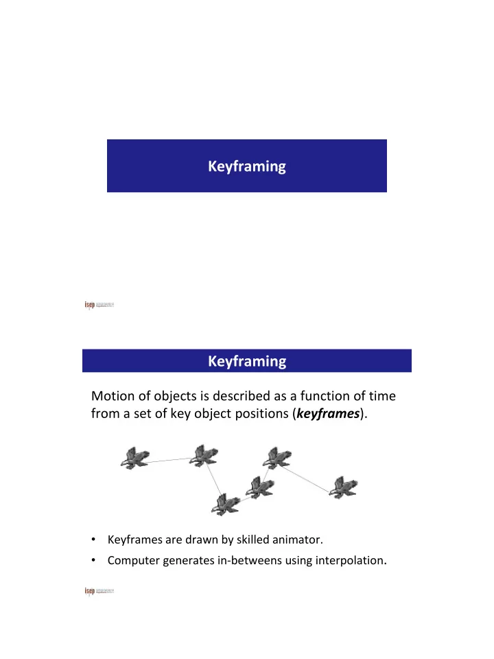
Motion of objects is described as a function of time from a set of key object positions (keyframes).

• Keyframes are drawn by skilled animator.
• Computer generates in-betweens using interpolation.

( ) s t

04-05-2017 2

Keyframing

Complex movements may require multiple keys.

Slide 4

Interpolating Positions

Given positions: find curve such that

( , , ), 0, ,

i i i

x y t i n         ( ) ( ) ( ) x t t y t C        ( )

i i i

x t y C

u

( , , ) x y t

1 1 1

( , , ) x y t

2 2 2

( , , ) x y t ( ) t C

04-05-2017 3 Lecture 10 Slide 5 6.837 Fall 2003

Linear Interpolation

Simple problem: Any ti:

( , , ) x y t

1 1 1

( , , ) x y t

2 2 2

( , , ) x y t



1 1 1 1 1 2 1 1 2 1 2 2 1 2 1

, , ( ) , , t t t t x x t t t t t t t x t t t t t x x t t t t t t t                          

1

=0 and =1 t t

 

  

1

( ) 1 x t x t x t Lecture 10 Slide 6 6.837 Fall 2003

Polynomial Interpolation

An n-degree polynomial can interpolate any n+1 points. The n+1 coefficients of an n-degree polynomial can be

• btained from the n+1 points.

( , , ) x y t

1 1 1

( , , ) x y t

2 2 2

( , , ) x y t

parabola

04-05-2017 4 Lecture 10 Slide 7

Spline Interpolation

For large number of points (N), many polynomials

• f small degree can be used.

Polynomials of small degree are faster and easier to control.

 

x t t t t 8-degree polynomial spline spline vs. polynomial Lecture 10

Spline Interpolation

A cubic polynomial between each pair of points: 4 parameters (degrees of freedom) for each spline segment. Input parameters: 4 points 2 points + 2 directions

2 3 1 2 3

( ) x t c c t c t c t    

04-05-2017 5 Lecture 10 Slide 12 6.837 Fall 2003

Interpolating Key Frames

• Interpolation is not fool proof.
• The splines may undershoot and cause interpenetration.
• The animator must solve these types of side-effects.

Keyframing

Keyframe animation can be applied to different parameters Parameter to interpolate:

position,

• rientation,

deformation, lights, camera,

• pacity?

04-05-2017 6

Physics Simulation

04-05-2017 7

Physics Simulation

Particles Rigid bodies Deformable bodies Fluid dynamics Vehicle dynamics Characters

Definitions

Kinematics: The study of motion without consideration of the underlying forces Dynamics: Study of physical motion (or more abstractly, the study of change in physical systems) Forward Dynamics: Computing motion resulting from applied forces Inverse Dynamics: Computing forces required to generate desired motion Mechanics, Statics, Kinetics

04-05-2017 8

Particles Particula

p(t) p(t+ t)

z y x

p p p , ,  p

04-05-2017 9

Kinematics of Particles

Position : x Velocity: v = dx/dt Acceleration: a = dv/dt = d2x/dt2



 dt v x

Aproximações númericas

Exato se v0 não varia em [0, t] Exato se v(t) não varia em t

t v x t x    ) ( t t v t t x t x       ) ( ) ( ) (

04-05-2017 10

Aceleração

Acceleration a=a0 Velocity Position

2

x v a 2 1 v x v a a v       

 

t t dt t dt

Aproximações númericas

Exato se a não varia em [0, t] Exato se a(t) não varia em t

2

) ( 2 1 ) ( ) ( ) ( t t a t t v t t x t x         

2

2 1 ) ( t a t v x t x

• 

   

04-05-2017 11

Forces

Multiple forces can add up to a single total force: Forces cause change in momentum (accelerations)

M /

total i total

f a f f  

Gravity

Gravity near Earth’s surface is constant: f=m.g (g = -9.8 m/s2) Gravity for distant objects: f=Gm1m2/r2 (G=6.673×10-11 m3/kg·s2)

04-05-2017 12

Spring-Damper

Spring: f = -kx k=spring constant x=distance from rest state Damper: f=-cv c=damping factor v=velocity along spring axis Spring-damper: f=-kx-cv

Aerodynamic Drag

Drag force: f=(1/2)ρaccdv2 ρ=fluid density ac=cross sectional area cd=coefficient of drag (geometric constant based on shape of object, usually between 0 and 1, but can be higher) v=velocity of the object relative to velocity of the fluid Note: for simple cases, (1/2)ρaccd is constant

04-05-2017 13

Friction

Static friction: f ≤ fnμs Dynamic friction: f = fnμd fn=normal force μs=coefficient of static friction μd=coefficient of dynamic friction

Force Fields

Generic force fields can be created that use arbitrary rules to define a force at some location: f=f(x) Examples: vortex, attractors, turbulence, torus…

04-05-2017 14

Collisions: Impulse

Momentum: p = m.v Impulse: J=Δp An impulse is a finite change in momentum Impulses are essentially large forces acting over a small time Modified momentum update: p=p0+fΔt+J  p/m = p0/m+fΔt/m+J/m  v = v0+aΔt+J/m

[kg.m.s-1] or [N.s]

Particle Simulation 1

Particle struct { Vector3d Velocity; Vector3d Position; float Mass; }

UpdateParticle(float dtime) {

Force = ComputeTotalForce(); Acel = Force/Mass; Velocity = Velocity + Acel * dtime; Position = Position + Velocity * dtime;

}

04-05-2017 15

Particle Simulation 2

Particle struct { Vector3d Momentum; Vector3d Position; float Mass; }

UpdateParticle(float dtime) {

Impulse = ComputeTotalImpulse(dtime); Momentum = Momentum + Impulse; Velocity = Momentum / Mass; Position = Position + Velocity * dtime;

}

Integration

Explicit Euler method: v=v0+aΔt x=x0+vΔt Other methods:

Implicit Euler Runge-Kutta Crank-Nicholson Multipoint Leapfrog DuFort-Frankel Adams, Adams-Moulton, Adams-Bashforth

Optimize for:

• Stability
• Accuracy
• Convergence
• Performance

04-05-2017 16

Rigid Bodies Angular Speed

lim

t d t dt   

 

   

• The average angular speed,

ωavg, of a rotating rigid

• bject is the ratio of the

angular displacement to the time interval

• The instantaneous angular

speed is defined as the limit of the average speed as the time interval approaches zero

• f

i avg f i

t t t          

04-05-2017 17

Instantaneous Angular Acceleration

lim

t d t dt   

 

   

• The instantaneous angular

acceleration is defined as the limit of the average angular acceleration as the time goes to 0

• SI Units of angular acceleration: rad/s²

Torque

• Torque, t , is tendency of a force to rotate object about some axis
• Torque is vector: Direction determined by axis of twist

t  Fd

F is the force d is the lever arm (or moment arm) Units are Newton m Φ is the angle between F and r

t  Frsin t  Fd

04-05-2017 18

Offset Forces

Torque resulting from offset force: τ=r×f Total force: Total torque:





i

f fres ) f r (

i i



 

res

t

Rotational Inertia

• Rotational inertia or moment of inertia I is the

resistance of an object to changes in its rotational motion.

• Rotational inertia I is the rotational equal of mass M.
• Rotational inertia depends on:
• Mass
• Distribution of that mass around the axis of rotation.

Units: kg·m2

I = ⌠ ⌡ r2 dm

04-05-2017 19

Moments of Inertia Rotational Inertia

                

zz zy zx yz yy yx xz xy xx

I I I I I I I I I I

 

   dm xy dm z y

xy xx

) ( I ) ( I

2 2

          

zz yy xx

I I I I0

T

A I A I

0

 

For arbitrary axis: A=3x3 orientation matrix

04-05-2017 20

Torque and Rotational Inertia

• Torque T is the application of a force which

changes the angular acceleration of the

• bject.

Newton’s Second Law for Rotation:

   I T

L  I L  mvr  mr2

Angular Momentum

Analogy between L and p

Angular Momentum Linear momentum L = Iw p = mv t = dL/dt t = I .  F = dp/dt F = m.a

Conserved if no net

• utside torques

Conserved if no net outside forces

Rigid body Point particle

04-05-2017 21

Angular Momentum

L=Iω = AI0ATω L=angular momentum I=rotational inertia ω=angular velocity A=3x3 orientation matrix

Rigid Body Simulation

RigidBody struct { Vector Position; Vector Velocity; Vector Orientation; Vector AngVelocity; float Mass; Matrix RotationInertia; } UpdateRigidBody(float dtime) { Force=ComputeTotalForce(); Torque=ComputeTotalTorque(); Aceleration = Force / Mass; Velocity = Velocity + Aceleration * dtime; Position = Position + Velocity * dtime; AngAceleration = Torque * Inverse(RotationalInertia); AngVelocity = AngVelocity + AngAceleration * dtime; Orientation = Orientation + AngVelocity * dtime; }

04-05-2017 22 http://bulletphysics.org/

• Physics Engine

– particle – rigid body – soft body

• Created by Erwin Coumans (previously of Sony)
• Professional-grade library
• Open Source
• Free for commercial use

Bullet3D

04-05-2017 23

• Continuous & Discrete Collision
• Ray & Convex Sweep Test
• Flexible Algorithm Selection System. Ex:

– Broad Phase: Sweep & Prune – Narrow Phase: GJK

Physics Features

• Concave & Convex Meshes
• All basic Primitives

Collision Shapes

04-05-2017 24

• Rigid body dynamics constraint solver
• Vehicle dynamics
• Character controller & solver
• Ragdoll physics
• Soft body dynamics

– cloth – rope – deformable volumes

Advanced Features

• Blender3D
• Maya
• And support for multiple formats:

– Collada (.dae) – Wavefront (.obj)

Integrated with various tools

04-05-2017 25

Bullet3D Components

• Perform collision detection
• Resolve collisions & other constraints
• Provide objects' updated world transform

Physics Engine Obligations

04-05-2017 26

• #include btBulletDynamicsCommon.h
• include Bullet/src path (-L …)
• build using these libs:

– BulletDynamics – BulletCollision – LinearMath

Bullet Setup

• Create a Bullet World
• Create a Rigid Body
• Create a Collision Object
• Update the simulation each frame
• Use object's world transform to render

Default Use of Bullet3D

04-05-2017 27

• Look at Hello World Demo
• Create:

– btDiscreteDynamicsWorld – btcollisionShape – btMotionState – btRigidBody

• Each frame:

– call stepSimulation on dynamic world – use world transform to render your object

Integrating Bullet in your App

• btDiscreteDynamicsWorld

OR

• BtSoftRigidDynamicsWorld
• Both subclasses of:

– btDynamicsWorld

• What does a world do?

– manages your physics objects & constraints – implements the update of all objects each frame

Create a Bullet World

04-05-2017 28

• Add it to the btDynamicsWorld

Create a Rigid Body

• btCollisionObject
• Provide:

– mass (0 if static) – collision shape – material properties

• frictional coefficient
• coefficient of restitution

Create a Collision Object

04-05-2017 29

• Plane
• Box
• Sphere
• Cone
• Convex Hull
• Triangle Mesh

Collision Shape Options Selecting the Best Bullet3D Collision Shape

04-05-2017 30

• Call stepSimulation

– will do frame's physics – updates the world transform for active objects

• via their btMotionState's setWorldTransform

– uses internal fixed timestep of 60Hz – performs interpolation for variation

Update the simulation each frame

• World Transform contains:

– position – orientation

Use Object's World Transform to Render

04-05-2017 31

• btScalar: - float

– define BT_USE_DOUBLE_PRECISION to use as double

• btVector3

– x,y,z,w – for 3D positions and vectors

• btQuaternion & btMatrix3x3

– for 3D orientations & rotations

Basic Bullet Data Types

• btCollisionObject

– a world transform – a collision shape

• btCollisionShape

– box, sphere, convex hull, triangle mesh – a single collision shape can be shared among multiple collision objects

• btCollisionWorld

– stores all collision objects

Key Collision Data Structures

04-05-2017 32

• Minimum Separation

– creates small gap

• Bullet3D uses 0.04

– 4 cm – can be changed, but don't set to 0

Collision Margin