
SLIDE 1
The Metric Dimension Problem.
- J. D´
ıaz
Monash U., May 2018
The Metric Dimension Problem. J. D az Monash U., May 2018 The - - PowerPoint PPT Presentation
The Metric Dimension Problem. J. D az Monash U., May 2018 The Metric Dimension problem Given G ( V , E ) its metric dimension, ( G ) is the cardinality of the smallest L V s.t. x , y V , z L with d G ( x , z ) = d
Monash U., May 2018
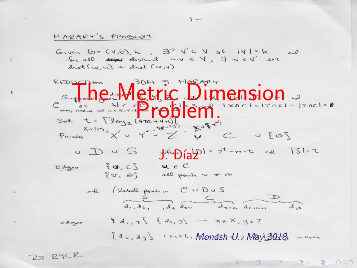
Given G(V , E) its metric dimension, β(G) is the cardinality of the smallest L ⊂ V s.t. ∀x, y ∈ V , ∃z ∈ L with dG(x, z) = dG(y, z). The set L is called a resolving set. Harary, Melter, (1976), Slater, (1974)
(4,3,0) (2,1,2) (4,1,4) (3,2,1) (1,2,3) (0,3,4) (3,0,3)
Given G(V , E) its metric dimension, β(G) is the cardinality of the smallest L ⊂ V s.t. ∀x, y ∈ V , ∃z ∈ V with dG(x, z) = dG(y, z). The set L is called a resolving set. Harary, Melter, (1976), Slater, (1974)
(4,0) (1,3) (2,2) (3,3) (3,1) (4,4) (0,4)
Khuller,Raghavachari,Rosenfeld (1996)
fathers of L with degree ≥ 3 ⇒ β(T) = |L| − |F|. (Slater 1975)
F L
For different examples of G and H produce UB and LB to the MD of G✷H. They gave an example of a G with bounded MD, where G✷G has unbounded MD. Caceres,Hernandez,Mora,Pelayo,Puertas,Sera,D.Wood (2007)
Khuller,Raghavachari,Rosenfeld (1996)
the authors determine the max. number of vertices for G ∈ Gβ,D. Hernando,Mora,Pelayo,Seara,Wood (2010)
D´ ıaz, Pottonen, Serna, Van Leeuwen, (2012)
Hoffman, Wanke (2012) G is Gabriel ∀u, v ∈ V (G) are adjacent if the closed disc of which line segment uv is diameter contains no w ∈ V (G). ⇒ Unit Disks Graphs are NPC
Epstein, Levin, Woeginger (2012)
Consider the 1-Negative Planar 3-SAT problem: Given a sat formula φ s.t.
◮ every variable occurs exactly once negatively and once or
twice positively,
◮ every clause contains two or three distinct variables, ◮ every clause with three distinct variables contains at least one
negative literal,
◮ the clause-variable graph Gφ is planar.
decide if it is SAT. 1-Negative Planar 3-SAT problem is NPC: reduction from Planar-SAT. 1-Negative Planar 3-SAT problem ≤p decisional MD bounded degree planar graphs.
Beliova,Eberhard,Erlebach,Hall,Hoffmann,Mih´ alak,Ram (2006)
NP⊆ DTIME (nlog log n), Hauptmann,Scmhied,Viehmann(12)
maximum degree 3, Hartung,Nichterlein (2013)
An undirected G is said to be an
plane without crossings in such a way that all of the vertices belong to the unbounded face of the drawing. For k > 1, G is said to be an k-outerplanar graph if removing the vertices on the outer face results in a (k − 1)-outerplanar embedding.
G and the edges in T correspond to inner edges and bridges (separators) of G. Notice as size of an inner face could be arbitrarily large, the width of T could be arbitrary. Explore T in bottom-up fashion using two data structures:
2.1 Boundary conditions 2.2 Configurations
Even the number of vertices in G represented by v ∈ V (T) could be unbounded, the total number of configurations is polynomial. The algorithm works in O(n8) (plenty of room for possible improvement)
Baker’s Technique (1994): The technique aims to produce FPTAS for problems that are known to be NPC on planar graphs. They decompose the planar realization into k-outerplanar, get an exact solution for each k-outerplanar slice and combine them. Solving for each k-outerplanar using DP on a tree decomposition, that for each vertex separator of size at most 2k.
tor PTAS in planar graphs ∈ PTAS for planar graphs. Is it in APX-hard?
away.
e b f g a c d e b f g a c d
A problem is bidimensional if it does not increase when performing certain operations as contraction of edges, and the solution value for the problem on a n × n-grid is Ω(n2) Demaine, Fomin, Hajiaghayi, Thilikos (2005) Bidimensionality has been used as a tool to find PTAS for bidimensional problems that are NPC on planar graphs. Demaine, Hajiaghayi (2005). Examples: feedback vertex set, minimum maximal matching, face cover, edge dominating set . . ..
The Tree-width of G = (V , E) is a tree ({Xi}, T}):
◮ ∪Xi = V ◮ ∀e ∈ E, ∃i : e ∈ Xi ◮ If v ∈ Xi ∩ Xj then ∀Xk ∈ Xi ❀ Xj we have v ∈ Xk
The tree width of a graph G is the size of its largest set |Xi| − 1.
Treewidth = 2 b a c d g f e abc cde efd fg
Classify the problems according to their difficulty with respect to the input size n an input parameter k of the problem. Downey, Fellows (1999) Fixed parameter tractable: FPT is the class of problems solvable in time f (k)poly(n) (where f (k) = 2k)
Time of k-VC = (kn + 1.2k). ∴ k-VC ∈ FPT.
checked in time O(m2k). P ⊆ FPT ⊆ W[1] ⊆ W[2] ⊆ · · · ⊆ XP
Courcelle’s Theorem Any problem definable by Monadic Second Order Logic is FPT when parametrized by tree width and the length of the formula. So far, it seems to be difficult to formulate MD as an MSOL-formula ⇒ Courcelle’s Theorem can’t apply.
MSOL formula.
graphs.
G ∈ G(n, p) if given n vertices V (G), each possible edge e is included independently with probability p = p(n). Whp |E(G)| = p n
2
Giant component threshold: pt = (1 + ǫ) 1
n.
Connectivity threshold: pc = (1 + ǫ) log n
n .
Bollobas, Mitsche, Pralat (2013) Given G ∈ G(n, p), choose randomly the resolving set L ⊆ V and bound Pr [∃u, v not separated by L].
d = np β
log5 n Θ(n) n1/2 log n n1/3 log n n1/4 log n log n log n Θ(1)
logc n
n1/5 n1/3 n1/4 n1/2 n(1 − ǫ)
G ∈ G(n, t) if it is uniformly sampled from the set of all graphs with n vertices and degree t. Assume t = Θ(1). Let G ∈ G(n, t):
◮ For t ≥ 3 aas G is strongly connected Cooper (93). ◮ For t ≥ 3 aas G is Hamiltonian Robinson,Wormald (92,93),
Cooper, Frieze (94).
◮ For t ≥ 3 aas the diameter of G = logt−1 +o(log n) Bollobas,
Fernandez de la Vega (81)
◮ For t ≥ 3, G is an expander, i.e. ∃c > 1 s.t. ∀S ⊂ V (G) with
1 ≤ |S| ≤ n
2, N (S) ≥ c|S|.
Given G ∈ G(n, t), |V | = n and 2 < t = Θ(1), then whp E [β(G)] = Θ(log n) Given G ∈ G(n, t), v ∈ V (G), let Si = {u ∈ V (G) | dG(v, u) = i}
(with 0 < α < 1) S1(v) S2(v)S3(v) Si(v) v
t
αin αi+1n
t(t − 1)3
i = logt−1 n
2
t(t − 1) Θ(√n) t(t − 1)2
Given v ∈ V (G), for any pair (u, w) ∈ V 2: v does not separate u and w if u, w ∈ Si, and v separates u and w if u ∈ Si & w ∈ Si+1 (or vice versa).
Therefore, Pr [v separates u&w] ≥ 2αiαi+1, and Pr [v does not separate u&v] ≥ α2
i + α2 i+1,
where αi and αi+1 are constants between 0 and 1. (1 − αiαi+1)
≥ Pr [v separates u&w] ≥ 2αiαi+1
α′
Randomly choose a resolving L ⊂ V (G) with |L| = C log n, for large constant C > 0. Then for a particular pair of vertices u, w Pr [L does not separate u&w] < αC log n ∼ o( 1
n2 ) (union bound)
Let XC = be the number of pairs not separated by L, E [XC] < n2αC log n → 0 ⇒ Pr [XC > 0] → 0
Randomly choose a resolving set L ⊂ V (G) with |L| = c log n, for small constant c > 0. Pr [L does not separate u&w] ≥ α′c log n ∼ ω( 1
n2 )
⇒ If Xc = number pairs not separated by L, then E [Xc] > n2α′c log n → ∞ ⇒ Pr [Xc > 0] = 1 − o(1) Therefore, β(G) = Θ(log n) .
For t = 3, empirically β(G) = 1.13 log n.
Given a square Q = [0, √n]2 and a real r(n) > 0 define a random geometric graph G ∈ G(n, r) by scattering n expected vertices V on Q according to a Poisson distribution with intensity 1, and for any u, v ∈ V , (u, v) ∈ E iff dE(u, v) ≤ r. It is known: (1) The giant component appears at rt = Θ(1). (2) There is a sharp connectivity threshold at rc = Θ√log n. (3) For v ∈ V , the expected degree d(v) = π log n.
Given G ∈ G(n, r(n)) what can we say about E [β]? If rt = O(1) ⇒ β(G) = Θ(n) Given v, u ∈ V (G) how can they be separated?
Let G ∈ G(n, rc) and let u, v ∈ V (G)2 with dE(u, v) = x Define the crowns: Ci(u, v) := {w ∈ V (G) : dE(u, w) = i and dE(v, w) = i + 1}
2r x r C1 C1 C2 C2 v u
LB: Compute the number of pairs for which C1 = ∅. Area of C1 = 4xrc ⇒ Pr [C1 = ∅] = e−4xrcn Number of (u, v) with C1 = ∅ is 2πn2 r
0 xe−4xrcndx = n log n
UB: Let x0 =
c
√
n(log n)1/3
Divide the pairs (u, v) in two groups : those with x ≤ x0 and the remaining ones. For the first group, E [|(u, v) ≤ x0|] = O(
n (log n)1/3 )
For the second group choose a random resolving L ⊆ V (G), with |L| =
n (log n)1/3 ,
If d(u, v) > x there are sufficiently large numbers of crowns each with enough vertices assure us each Ci(u, v) intersects L. Therefore at rc = Θ(
n ):
n log n ≤ β(G) ≤ n log1/3 n
What we know and don’t know:
◮ If r = O(1) ⇒ β(G) = Θ(n) ◮ If 1 << r << √log log n ⇒ β(G) = Θ(ne−πr2) ◮ If r = C√log n ⇒ n log n ≤ β(G) ≤ n log1/3 n ? ◮ If log n ≤ r ≤ (n log3 n)1/4 ⇒ n r2 ≤ β(G) ≤ n log2 n r2
?
◮ If (n log1/3 n)1/4 ≤ r ≤ √n 4 ⇒ β(G) = Θ(r2/3n1/3) ? ◮ If r ≥ √n √ 2 ⇒ β(G) = Θ(n) ?