
SLIDE 1
Welcome back... Metric spaces.
A metric space X, d(i,j) where d(i,j) ≤ d(i,k)+d(k,j), d(i,j) = d(j,i), and d(i,j) ≥ 0. Which are metric spaces? (A) X from Rd and d(·,·) is Euclidean distance. (B) X from Rd and d(·,·) is squared Euclidean distance. (C) X- vertices in graph, d(i,j) is shortest path distances in graph. (D) X is a set of vectors and d(u,v) is u ·v. Input to TSP , facility location, some layout problems, ..., metric labelling. Hard problems. Easier to solve on trees. Dynamic programming on trees. Approximate metric on trees?
Approximate metric using a tree.
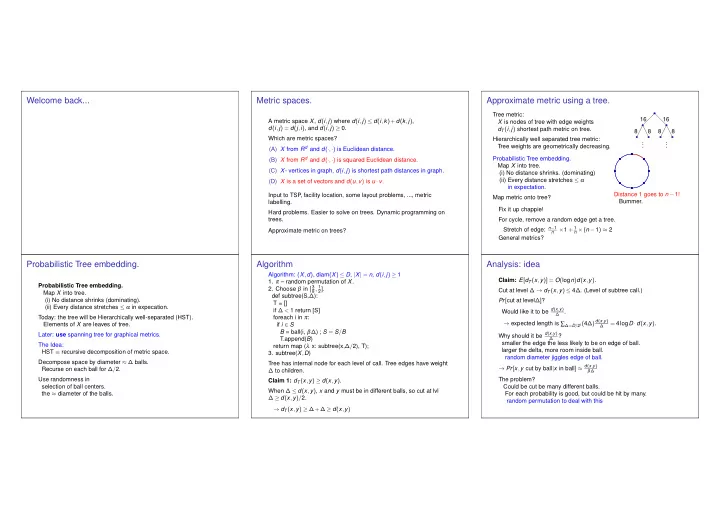
Tree metric: X is nodes of tree with edge weights dT (i,j) shortest path metric on tree. Hierarchically well separated tree metric: Tree weights are geometrically decreasing. 16 16 8 8 8 8 . . . . . . Probabilistic Tree embedding. Map X into tree. (i) No distance shrinks. (dominating) (ii) Every distance stretches ≤ α in expectation. Map metric onto tree? Distance 1 goes to n −1! Bummer. Fix it up chappie! For cycle, remove a random edge get a tree. Stretch of edge: n−1
n
×1 + 1
n ×(n −1) ≈ 2
General metrics?
Probabilistic Tree embedding.
Probabilistic Tree embedding. Map X into tree. (i) No distance shrinks (dominating). (ii) Every distance stretches ≤ α in expecation. Today: the tree will be Hierarchically well-separated (HST). Elements of X are leaves of tree. Later: use spanning tree for graphical metrics. The Idea: HST ≡ recursive decomposition of metric space. Decompose space by diameter ≈ ∆ balls. Recurse on each ball for ∆/2. Use randomness in selection of ball centers. the ≈ diameter of the balls.
Algorithm
Algorithm: (X,d), diam(X) ≤ D, |X| = n, d(i,j) ≥ 1
- 1. π – random permutation of X.
- 2. Choose β in [ 3
8, 1 2].
def subtree(S,∆): T = [] if ∆ < 1 return [S] foreach i in π: if i ∈ S B = ball(i, β∆) ; S = S/B T.append(B) return map (λ x: subtree(x,∆/2), T);
- 3. subtree(X,D)
Tree has internal node for each level of call. Tree edges have weight ∆ to children. Claim 1: dT (x,y) ≥ d(x,y). When ∆ ≤ d(x,y), x and y must be in different balls, so cut at lvl ∆ ≥ d(x,y)/2. → dT (x,y) ≥ ∆+∆ ≥ d(x,y)
Analysis: idea
Claim: E[dT (x,y)] = O(logn)d(x,y). Cut at level ∆ → dT (x,y) ≤ 4∆. (Level of subtree call.) Pr[cut at level∆]? Would like it to be d(x,y)
∆
. → expected length is ∑∆=D/2i (4∆) d(x,y)
∆
= 4logD ·d(x,y). Why should it be d(x,y)
∆