
SLIDE 1
Joint Distributions, Independence Covariance and Correlation 18.05 Spring 2014
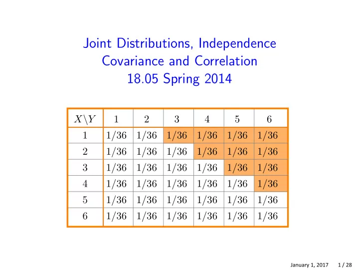
X\Y 1 2 3 4 5 6 1 1/36 1/36 1/36 1/36 1/36 1/36 2 1/36 1/36 1/36 1/36 1/36 1/36 3 1/36 1/36 1/36 1/36 1/36 1/36 4 1/36 1/36 1/36 1/36 1/36 1/36 5 1/36 1/36 1/36 1/36 1/36 1/36 6 1/36 1/36 1/36 1/36 1/36 1/36
January 1, 2017 1 / 28