Unit 6: Introduction to linear regression MT 2 scores posted in - - PowerPoint PPT Presentation

Unit 6: Introduction to linear regression

• 1. Introduction to regression

Sta 101 - Fall 2017

Duke University, Department of Statistical Science

• Dr. Mukherjee

Slides posted at http://www2.stat.duke.edu/courses/Fall17/sta101.002/

Announcements ▶ MT 2 scores posted in Sakai! ▶ Start working on your Final projects.

Due date- Sunday Dec 3, 11:55 PM.

– Lab:10:05 AM, 11:45 AM and 1:25 PM will present on Dec 4 during their Lab session. No lab on Monday for 8:30 AM and 3:05 PM. – Lab: 8:30 AM and 3:05 PM will present on Dec 5 during our lecture at Social Science 139. Your labs TAs will be here! No lecture on Tuesday for 10:05 AM, 11:45 AM and 1:25 PM.

▶ PS 6 due date Nov 17 at 11:55 PM. ▶ PA 6 due date Nov 19 at 11:55 PM.

1

Modeling numerical variables ▶ So far we have worked with single numerical and categorical

variables, and explored relationships between numerical and categorical, and two categorical variables.

▶ In this unit we will learn to quantify the relationship between two

numerical variables, as well as modeling numerical response variables using a numerical or categorical explanatory variable.

▶ In the next unit we’ll learn to model numerical variables using

many explanatory variables at once.

2

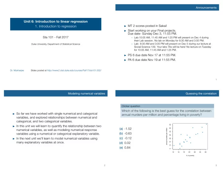
Guessing the correlation

Clicker question

Which of the following is the best guess for the correlation between annual murders per million and percentage living in poverty? (a) -1.52 (b) -0.63 (c) -0.12 (d) 0.02 (e) 0.84

• 14

16 18 20 22 24 26 5 10 15 20 25 30 35 40 % in poverty annual murders per million

3

Guessing the correlation

Clicker question

Which of the following is the best guess for the correlation between annual murders per million and population size? (a) -0.97 (b) -0.61 (c) -0.06 (d) 0.55 (e) 0.97

• 2e+06

4e+06 6e+06 8e+06 5 10 15 20 25 30 35 40 population annual murders per million

4

Assessing the correlation

Clicker question

Which of the following is has the strongest correlation, i.e. correlation coefficient closest to +1 or -1?

• (a)
• (b)
• (c)
• (d)

5

Spurious correlations

Remember: correlation does not always imply causation! http://www.tylervigen.com/

6

(2) Least squares line minimizes squared residuals ▶ Residuals are the leftovers from the model fit, and calculated as

the difference between the observed and predicted y: ei = yi − ˆ yi

▶ The least squares line minimizes squared residuals:

– Population data: ˆ y = β0 + β1x – Sample data: ˆ y = b0 + b1x

• 14

16 18 20 22 24 26 5 10 15 20 25 30 35 40 % in poverty annual murders per million

7

(3) Interpreting the last squares line ▶ Slope: For each unit increase in x, y is expected to be

higher/lower on average by the slope. b1 = sy sx R

▶ Intercept: When x = 0, y is expected to equal the intercept.

b0 = ¯ y − b1¯ x

– The calculation of the intercept uses the fact the a regression line always passes through (¯ x,¯ y).

8

Why does the regression line always pass through (¯ x,¯ y)?

▶ If there is no relationship between x and y (b1 = 0), the best

guess for ˆ y for any value of x is ¯ y.

▶ Even when there is a relationship between x and y (b1 ̸= 0), the

best guess for ˆ y when x = ¯ x is still ¯ y.

−1.0 0.0 0.5 1.0 1.5 2.0 −1.5 −0.5 0.5 1.5 x y

• (x, y)

−1.0 0.0 0.5 1.0 1.5 2.0 −2 2 4 x y2

• (x, y)

−1.0 0.0 0.5 1.0 1.5 2.0 −2 2 4 6 8 10 x y3

• (x, y)

9

Application exercise: 6.1 Linear model

See course website for details

10

Clicker question

What is the interpretation of the slope? (a) Each additional percentage in those living in poverty increases number of annual murders per million by 2.56. (b) For each percentage increase in those living in poverty, the number of annual murders per million is expected to be higher by 2.56 on average. (c) For each percentage increase in those living in poverty, the number of annual murders per million is expected to be lower by 29.91 on average. (d) For each percentage increase annual murders per million, the percentage of those living in poverty is expected to be higher by 2.56 on average.

11

Clicker question

Suppose you want to predict annual murder count (per million) for a series of districts that were not included in the dataset. For which of the following districts would you be most comfortable with your prediction? A district where % in poverty = (a) 5% (b) 15% (c) 20% (d) 26% (e) 40%

• 14

16 18 20 22 24 26 5 10 15 20 25 30 35 40 % in poverty annual murders per million

12

A note about the intercept

Sometimes the intercept might be an extrapolation: useful for adjusting the height of the line, but meaningless in the context of the data.

10 20 30 40 50 60 −40 40 80 % in poverty annual murders per million

• 13

Calculating predicted values

By hand: murder = −29.91 + 2.56 poverty The predicted number of murders per million per year for a county with 20% poverty rate is:

• murder = −29.91 + 2.56 × 20 = 21.29

In R:

# load data murder <- read.csv("https://stat.duke.edu/~mc301/data/murder.csv") # fit model m_mur_pov <- lm(annual_murders_per_mil ~ perc_pov, data = murder) # create new data newdata <- data.frame(perc_pov = 20) # predict predict(m_mur_pov, newdata) 1 21.28663 14

Summary of main ideas

• 1. Correlation coefficient describes the strength and direction of

the linear association between two numerical variables

• 2. Least squares line minimizes squared residuals
• 3. Interpreting the least squares line
• 4. Predict, but don’t extrapolate

15