Linear regression Linear regression is a simple approach to - - PowerPoint PPT Presentation

Linear regression

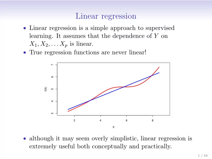
• Linear regression is a simple approach to supervised
• learning. It assumes that the dependence of Y on

X1, X2, . . . Xp is linear.

• True regression functions are never linear!

2 4 6 8 3 4 5 6 7 X f(X)

• although it may seem overly simplistic, linear regression is

extremely useful both conceptually and practically.

1 / 48

Linear regression for the advertising data

Consider the advertising data shown on the next slide. Questions we might ask:

• Is there a relationship between advertising budget and

sales?

• How strong is the relationship between advertising budget

and sales?

• Which media contribute to sales?
• How accurately can we predict future sales?
• Is the relationship linear?
• Is there synergy among the advertising media?

2 / 48

Advertising data

50 100 200 300 5 10 15 20 25 TV Sales 10 20 30 40 50 5 10 15 20 25 Radio Sales 20 40 60 80 100 5 10 15 20 25 Newspaper Sales

3 / 48

Simple linear regression using a single predictor X.

• We assume a model

Y = β0 + β1X + ǫ, where β0 and β1 are two unknown constants that represent the intercept and slope, also known as coefficients or parameters, and ǫ is the error term.

• Given some estimates ˆ

β0 and ˆ β1 for the model coefficients, we predict future sales using ˆ y = ˆ β0 + ˆ β1x, where ˆ y indicates a prediction of Y on the basis of X = x. The hat symbol denotes an estimated value.

4 / 48

Estimation of the parameters by least squares

• Let ˆ

yi = ˆ β0 + ˆ β1xi be the prediction for Y based on the ith value of X. Then ei = yi − ˆ yi represents the ith residual

• We define the residual sum of squares (RSS) as

RSS = e2

1 + e2 2 + · · · + e2 n,

• r equivalently as

RSS = (y1−ˆ β0−ˆ β1x1)2+(y2−ˆ β0−ˆ β1x2)2+. . .+(yn−ˆ β0−ˆ β1xn)2.

• The least squares approach chooses ˆ

β0 and ˆ β1 to minimize the RSS. The minimizing values can be shown to be ˆ β1 = n

i=1(xi − ¯

x)(yi − ¯ y) n

i=1(xi − ¯

x)2 , ˆ β0 = ¯ y − ˆ β1¯ x, where ¯ y ≡ 1

n

n

i=1 yi and ¯

x ≡ 1

n

n

i=1 xi are the sample

means.

5 / 48

Example: advertising data

50 100 150 200 250 300 5 10 15 20 25 TV Sales

The least squares fit for the regression of sales onto TV. In this case a linear fit captures the essence of the relationship, although it is somewhat deficient in the left of the plot.

6 / 48

Assessing the Accuracy of the Coefficient Estimates

• The standard error of an estimator reflects how it varies

under repeated sampling. We have SE(ˆ β1)

2 =

σ2 n

i=1(xi − ¯

x)2 , SE(ˆ β0)

2 = σ2

1 n + ¯ x2 n

i=1(xi − ¯

x)2

• ,

where σ2 = Var(ǫ)

• These standard errors can be used to compute confidence
• intervals. A 95% confidence interval is defined as a range of

values such that with 95% probability, the range will contain the true unknown value of the parameter. It has the form ˆ β1 ± 2 · SE(ˆ β1).

7 / 48

Confidence intervals — continued

That is, there is approximately a 95% chance that the interval

• ˆ

β1 − 2 · SE(ˆ β1), ˆ β1 + 2 · SE(ˆ β1)

• will contain the true value of β1 (under a scenario where we got

repeated samples like the present sample) For the advertising data, the 95% confidence interval for β1 is [0.042, 0.053]

8 / 48

Hypothesis testing

• Standard errors can also be used to perform hypothesis

tests on the coefficients. The most common hypothesis test involves testing the null hypothesis of H0 : There is no relationship between X and Y versus the alternative hypothesis HA : There is some relationship between X and Y .

• Mathematically, this corresponds to testing

H0 : β1 = 0 versus HA : β1 = 0, since if β1 = 0 then the model reduces to Y = β0 + ǫ, and X is not associated with Y .

9 / 48

Hypothesis testing — continued

• To test the null hypothesis, we compute a t-statistic, given

by t = ˆ β1 − 0 SE(ˆ β1) ,

• This will have a t-distribution with n − 2 degrees of

freedom, assuming β1 = 0.

• Using statistical software, it is easy to compute the

probability of observing any value equal to |t| or larger. We call this probability the p-value.

10 / 48

Results for the advertising data

Coefficient

• Std. Error

t-statistic p-value Intercept 7.0325 0.4578 15.36 < 0.0001 TV 0.0475 0.0027 17.67 < 0.0001

11 / 48

Assessing the Overall Accuracy of the Model

• We compute the Residual Standard Error

RSE =

• 1

n − 2RSS =

• 1

n − 2

n

• i=1

(yi − ˆ yi)2, where the residual sum-of-squares is RSS = n

i=1(yi − ˆ

yi)2.

• R-squared or fraction of variance explained is

R2 = TSS − RSS TSS = 1 − RSS TSS where TSS = n

i=1(yi − ¯

y)2 is the total sum of squares.

• It can be shown that in this simple linear regression setting

that R2 = r2, where r is the correlation between X and Y : r = n

i=1(xi − x)(yi − y)

n

i=1(xi − x)2n i=1(yi − y)2 .

12 / 48

Advertising data results

Quantity Value Residual Standard Error 3.26 R2 0.612 F-statistic 312.1

13 / 48

Multiple Linear Regression

• Here our model is

Y = β0 + β1X1 + β2X2 + · · · + βpXp + ǫ,

• We interpret βj as the average effect on Y of a one unit

increase in Xj, holding all other predictors fixed. In the advertising example, the model becomes sales = β0 + β1 × TV + β2 × radio + β3 × newspaper + ǫ.

14 / 48

Interpreting regression coefficients

• The ideal scenario is when the predictors are uncorrelated

— a balanced design:

• Each coefficient can be estimated and tested separately.
• Interpretations such as “a unit change in Xj is associated

with a βj change in Y , while all the other variables stay fixed”, are possible.

• Correlations amongst predictors cause problems:
• The variance of all coefficients tends to increase, sometimes

dramatically

• Interpretations become hazardous — when Xj changes,

everything else changes.

• Claims of causality should be avoided for observational

data.

15 / 48

The woes of (interpreting) regression coefficients

“Data Analysis and Regression” Mosteller and Tukey 1977

• a regression coefficient βj estimates the expected change in

Y per unit change in Xj, with all other predictors held

• fixed. But predictors usually change together!
• Example: Y total amount of change in your pocket;

X1 = # of coins; X2 = # of pennies, nickels and dimes. By itself, regression coefficient of Y on X2 will be > 0. But how about with X1 in model?

• Y = number of tackles by a football player in a season; W

and H are his weight and height. Fitted regression model is ˆ Y = b0 + .50W − .10H. How do we interpret ˆ β2 < 0?

16 / 48

Two quotes by famous Statisticians

“Essentially, all models are wrong, but some are useful” George Box “The only way to find out what will happen when a complex system is disturbed is to disturb the system, not merely to

• bserve it passively”

Fred Mosteller and John Tukey, paraphrasing George Box

17 / 48

Estimation and Prediction for Multiple Regression

• Given estimates ˆ

β0, ˆ β1, . . . ˆ βp, we can make predictions using the formula ˆ y = ˆ β0 + ˆ β1x1 + ˆ β2x2 + · · · + ˆ βpxp.

• We estimate β0, β1, . . . , βp as the values that minimize the

sum of squared residuals RSS =

n

• i=1

(yi − ˆ yi)2 =

n

• i=1

(yi − ˆ β0 − ˆ β1xi1 − ˆ β2xi2 − · · · − ˆ βpxip)2. This is done using standard statistical software. The values ˆ β0, ˆ β1, . . . , ˆ βp that minimize RSS are the multiple least squares regression coefficient estimates.

18 / 48

X1 X2 Y

19 / 48

Results for advertising data

Coefficient

• Std. Error

t-statistic p-value Intercept 2.939 0.3119 9.42 < 0.0001 TV 0.046 0.0014 32.81 < 0.0001 radio 0.189 0.0086 21.89 < 0.0001 newspaper

• 0.001

0.0059

• 0.18

0.8599 Correlations: TV radio newspaper sales TV 1.0000 0.0548 0.0567 0.7822 radio 1.0000 0.3541 0.5762 newspaper 1.0000 0.2283 sales 1.0000

20 / 48

Some important questions

• 1. Is at least one of the predictors X1, X2, . . . , Xp useful in

predicting the response?

• 2. Do all the predictors help to explain Y , or is only a subset
• f the predictors useful?
• 3. How well does the model fit the data?
• 4. Given a set of predictor values, what response value should

we predict, and how accurate is our prediction?

21 / 48

Is at least one predictor useful?

For the first question, we can use the F-statistic F = (TSS − RSS)/p RSS/(n − p − 1) ∼ Fp,n−p−1 Quantity Value Residual Standard Error 1.69 R2 0.897 F-statistic 570

22 / 48

Deciding on the important variables

• The most direct approach is called all subsets or best

subsets regression: we compute the least squares fit for all possible subsets and then choose between them based on some criterion that balances training error with model size.

• However we often can’t examine all possible models, since

they are 2p of them; for example when p = 40 there are

• ver a billion models!

Instead we need an automated approach that searches through a subset of them. We discuss two commonly use approaches next.

23 / 48

Forward selection

• Begin with the null model — a model that contains an

intercept but no predictors.

• Fit p simple linear regressions and add to the null model

the variable that results in the lowest RSS.

• Add to that model the variable that results in the lowest

RSS amongst all two-variable models.

• Continue until some stopping rule is satisfied, for example

when all remaining variables have a p-value above some threshold.

24 / 48

Backward selection

• Start with all variables in the model.
• Remove the variable with the largest p-value — that is, the

variable that is the least statistically significant.

• The new (p − 1)-variable model is fit, and the variable with

the largest p-value is removed.

• Continue until a stopping rule is reached. For instance, we

may stop when all remaining variables have a significant p-value defined by some significance threshold.

25 / 48

Model selection — continued

• Later we discuss more systematic criteria for choosing an

“optimal” member in the path of models produced by forward or backward stepwise selection.

• These include Mallow’s Cp, Akaike information criterion

(AIC), Bayesian information criterion (BIC), adjusted R2 and Cross-validation (CV).

26 / 48

Other Considerations in the Regression Model

Qualitative Predictors

• Some predictors are not quantitative but are qualitative,

taking a discrete set of values.

• These are also called categorical predictors or factor

variables.

• See for example the scatterplot matrix of the credit card

data in the next slide. In addition to the 7 quantitative variables shown, there are four qualitative variables: gender, student (student status), status (marital status), and ethnicity (Caucasian, African American (AA) or Asian).

27 / 48

Credit Card Data

Balance

20 40 60 80 100 5 10 15 20 2000 8000 14000 500 1500 20 40 60 80 100

Age Cards

2 4 6 8 5 10 15 20

Education Income

50 100 150 2000 8000 14000

Limit

500 1500 2 4 6 8 50 100 150 200 600 1000 200 600 1000

Rating

28 / 48

Qualitative Predictors — continued

Example: investigate differences in credit card balance between males and females, ignoring the other variables. We create a new variable xi =

• 1

if ith person is female if ith person is male Resulting model: yi = β0 + β1xi + ǫi =

• β0 + β1 + ǫi

if ith person is female β0 + ǫi if ith person is male. Intrepretation?

29 / 48

Credit card data — continued

Results for gender model: Coefficient

• Std. Error

t-statistic p-value Intercept 509.80 33.13 15.389 < 0.0001 gender[Female] 19.73 46.05 0.429 0.6690

30 / 48

Qualitative predictors with more than two levels

• With more than two levels, we create additional dummy
• variables. For example, for the ethnicity variable we

create two dummy variables. The first could be xi1 =

• 1

if ith person is Asian if ith person is not Asian, and the second could be xi2 =

• 1

if ith person is Caucasian if ith person is not Caucasian.

31 / 48

Qualitative predictors with more than two levels — continued.

• Then both of these variables can be used in the regression

equation, in order to obtain the model

yi = β0+β1xi1+β2xi2+ǫi =      β0 + β1 + ǫi if ith person is Asian β0 + β2 + ǫi if ith person is Caucasian β0 + ǫi if ith person is AA.

• There will always be one fewer dummy variable than the

number of levels. The level with no dummy variable — African American in this example — is known as the baseline.

32 / 48

Results for ethnicity

Coefficient

• Std. Error

t-statistic p-value Intercept 531.00 46.32 11.464 < 0.0001 ethnicity[Asian]

• 18.69

65.02

• 0.287

0.7740 ethnicity[Caucasian]

• 12.50

56.68

• 0.221

0.8260

33 / 48

Extensions of the Linear Model

Removing the additive assumption: interactions and nonlinearity Interactions:

• In our previous analysis of the Advertising data, we

assumed that the effect on sales of increasing one advertising medium is independent of the amount spent on the other media.

• For example, the linear model
• sales = β0 + β1 × TV + β2 × radio + β3 × newspaper

states that the average effect on sales of a one-unit increase in TV is always β1, regardless of the amount spent

• n radio.

34 / 48

Interactions — continued

• But suppose that spending money on radio advertising

actually increases the effectiveness of TV advertising, so that the slope term for TV should increase as radio increases.

• In this situation, given a fixed budget of $100, 000,

spending half on radio and half on TV may increase sales more than allocating the entire amount to either TV or to radio.

• In marketing, this is known as a synergy effect, and in

statistics it is referred to as an interaction effect.

35 / 48

Interaction in the Advertising data?

Sales Radio TV

When levels of either TV or radio are low, then the true sales are lower than predicted by the linear model. But when advertising is split between the two media, then the model tends to underestimate sales.

36 / 48

Modelling interactions — Advertising data

Model takes the form sales = β0 + β1 × TV + β2 × radio + β3 × (radio × TV) + ǫ = β0 + (β1 + β3 × radio) × TV + β2 × radio + ǫ. Results: Coefficient

• Std. Error

t-statistic p-value Intercept 6.7502 0.248 27.23 < 0.0001 TV 0.0191 0.002 12.70 < 0.0001 radio 0.0289 0.009 3.24 0.0014 TV×radio 0.0011 0.000 20.73 < 0.0001

37 / 48

Interpretation

• The results in this table suggests that interactions are

important.

• The p-value for the interaction term TV×radio is

extremely low, indicating that there is strong evidence for HA : β3 = 0.

• The R2 for the interaction model is 96.8%, compared to
• nly 89.7% for the model that predicts sales using TV and

radio without an interaction term.

38 / 48

Interpretation — continued

• This means that (96.8 − 89.7)/(100 − 89.7) = 69% of the

variability in sales that remains after fitting the additive model has been explained by the interaction term.

• The coefficient estimates in the table suggest that an

increase in TV advertising of $1, 000 is associated with increased sales of (ˆ β1 + ˆ β3 × radio) × 1000 = 19 + 1.1 × radio units.

• An increase in radio advertising of $1, 000 will be

associated with an increase in sales of (ˆ β2 + ˆ β3 × TV) × 1000 = 29 + 1.1 × TV units.

39 / 48

Hierarchy

• Sometimes it is the case that an interaction term has a

very small p-value, but the associated main effects (in this case, TV and radio) do not.

• The hierarchy principle:

If we include an interaction in a model, we should also include the main effects, even if the p-values associated with their coefficients are not significant.

40 / 48

Hierarchy — continued

• The rationale for this principle is that interactions are hard

to interpret in a model without main effects — their meaning is changed.

• Specifically, the interaction terms also contain main effects,

if the model has no main effect terms.

41 / 48

Interactions between qualitative and quantitative variables

Consider the Credit data set, and suppose that we wish to predict balance using income (quantitative) and student (qualitative). Without an interaction term, the model takes the form

balancei ≈ β0 + β1 × incomei +

• β2

if ith person is a student if ith person is not a student = β1 × incomei +

• β0 + β2

if ith person is a student β0 if ith person is not a student.

42 / 48

With interactions, it takes the form

balancei ≈ β0 + β1 × incomei +

• β2 + β3 × incomei

if student if not student =

• (β0 + β2) + (β1 + β3) × incomei

if student β0 + β1 × incomei if not student

43 / 48

50 100 150 200 600 1000 1400 Income Balance 50 100 150 200 600 1000 1400 Income Balance student non−student

Credit data; Left: no interaction between income and student. Right: with an interaction term between income and student.

44 / 48

Non-linear effects of predictors

polynomial regression on Auto data

50 100 150 200 10 20 30 40 50 Horsepower Miles per gallon Linear Degree 2 Degree 5 45 / 48

The figure suggests that mpg = β0 + β1 × horsepower + β2 × horsepower2 + ǫ may provide a better fit. Coefficient

• Std. Error

t-statistic p-value Intercept 56.9001 1.8004 31.6 < 0.0001 horsepower

• 0.4662

0.0311

• 15.0

< 0.0001 horsepower2 0.0012 0.0001 10.1 < 0.0001

46 / 48

What we did not cover

Outliers Non-constant variance of error terms High leverage points Collinearity See text Section 3.33

47 / 48

Generalizations of the Linear Model

In much of the rest of this course, we discuss methods that expand the scope of linear models and how they are fit:

• Classification problems: logistic regression, support vector

machines

• Non-linearity: kernel smoothing, splines and generalized

additive models; nearest neighbor methods.

• Interactions: Tree-based methods, bagging, random forests

and boosting (these also capture non-linearities)

• Regularized fitting: Ridge regression and lasso

48 / 48