Introduction to Matlab (Code) Created by Stefan Roth, TU Darmstadt - PDF document

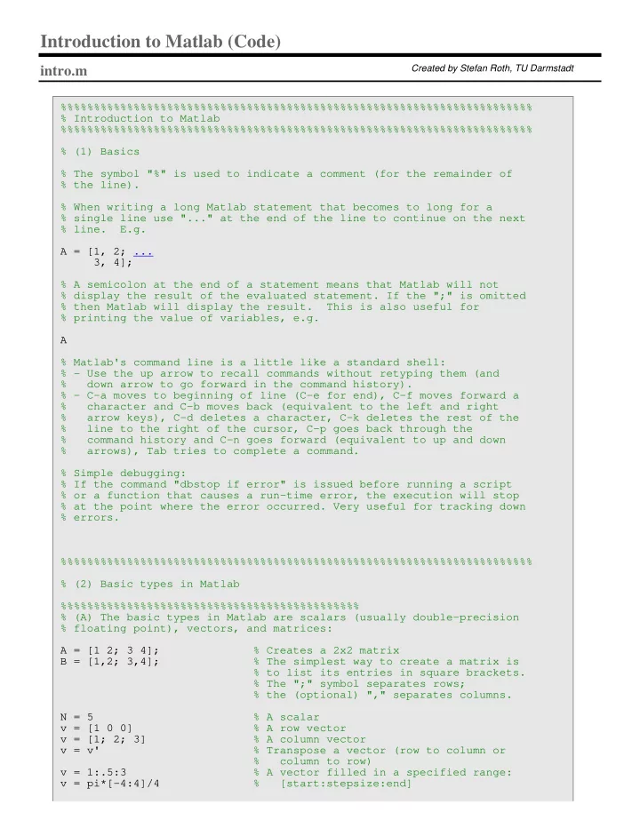
Introduction to Matlab (Code) Created by Stefan Roth, TU Darmstadt intro.m %%%%%%%%%%%%%%%%%%%%%%%%%%%%%%%%%%%%%%%%%%%%%%%%%%%%%%%%%%%%%%%%%%%%%%% % Introduction to Matlab %%%%%%%%%%%%%%%%%%%%%%%%%%%%%%%%%%%%%%%%%%%%%%%%%%%%%%%%%%%%%%%%%%%%%%% % (1) Basics % The symbol "%" is used to indicate a comment (for the remainder of % the line). % When writing a long Matlab statement that becomes to long for a % single line use "..." at the end of the line to continue on the next % line. E.g. A = [1, 2; ... 3, 4]; % A semicolon at the end of a statement means that Matlab will not % display the result of the evaluated statement. If the ";" is omitted % then Matlab will display the result. This is also useful for % printing the value of variables, e.g. A % Matlab's command line is a little like a standard shell: % - Use the up arrow to recall commands without retyping them (and % down arrow to go forward in the command history). % - C-a moves to beginning of line (C-e for end), C-f moves forward a % character and C-b moves back (equivalent to the left and right % arrow keys), C-d deletes a character, C-k deletes the rest of the % line to the right of the cursor, C-p goes back through the % command history and C-n goes forward (equivalent to up and down % arrows), Tab tries to complete a command. % Simple debugging: % If the command "dbstop if error" is issued before running a script % or a function that causes a run-time error, the execution will stop % at the point where the error occurred. Very useful for tracking down % errors. %%%%%%%%%%%%%%%%%%%%%%%%%%%%%%%%%%%%%%%%%%%%%%%%%%%%%%%%%%%%%%%%%%%%%%% % (2) Basic types in Matlab %%%%%%%%%%%%%%%%%%%%%%%%%%%%%%%%%%%%%%%%%%%%% % (A) The basic types in Matlab are scalars (usually double-precision % floating point), vectors, and matrices: A = [1 2; 3 4]; % Creates a 2x2 matrix B = [1,2; 3,4]; % The simplest way to create a matrix is % to list its entries in square brackets. % The ";" symbol separates rows; % the (optional) "," separates columns. N = 5 % A scalar v = [1 0 0] % A row vector v = [1; 2; 3] % A column vector v = v' % Transpose a vector (row to column or % column to row) v = 1:.5:3 % A vector filled in a specified range: v = pi*[-4:4]/4 % [start:stepsize:end]

% (brackets are optional) v = [] % Empty vector %%%%%%%%%%%%%%%%%%%%%%%%%%%%%%%%%%%%%%%%%%%%% % (B) Creating special matrices: 1ST parameter is ROWS, % 2ND parameter is COLS m = zeros(2, 3) % Creates a 2x3 matrix of zeros v = ones(1, 3) % Creates a 1x3 matrix (row vector) of ones m = eye(3) % Identity matrix (3x3) v = rand(3, 1) % Randomly filled 3x1 matrix (column % vector); see also randn % But watch out: m = zeros(3) % Creates a 3x3 matrix (!) of zeros %%%%%%%%%%%%%%%%%%%%%%%%%%%%%%%%%%%%%%%%%%%%% % (C) Indexing vectors and matrices. % Warning: Indices always start at 1 and *NOT* at 0! v = [1 2 3]; v(3) % Access a vector element m = [1 2 3 4; 5 7 8 8; 9 10 11 12; 13 14 15 16] m(1, 3) % Access a matrix element % matrix(ROW #, COLUMN #) m(2, :) % Access a whole matrix row (2nd row) m(:, 1) % Access a whole matrix column (1st column) m(1, 1:3) % Access elements 1 through 3 of the 1st row m(2:3, 2) % Access elements 2 through 3 of the % 2nd column m(2:end, 3) % Keyword "end" accesses the remainder of a % column or row m = [1 2 3; 4 5 6] size(m) % Returns the size of a matrix size(m, 1) % Number of rows size(m, 2) % Number of columns m1 = zeros(size(m)) % Create a new matrix with the size of m who % List variables in workspace whos % List variables w/ info about size, type, etc. %%%%%%%%%%%%%%%%%%%%%%%%%%%%%%%%%%%%%%%%%%%%%%%%%%%%%%%%%%%%%%%%%%%%%%% % (3) Simple operations on vectors and matrices %%%%%%%%%%%%%%%%%%%%%%%%%%%%%%%%%%%%%%%%%%%%%%%% % (A) Element-wise operations: % These operations are done "element by element". If two % vectors/matrices are to be added, subtracted, or element-wise % multiplied or divided, they must have the same size. a = [1 2 3 4]'; % A column vector 2 * a % Scalar multiplication a / 4 % Scalar division b = [5 6 7 8]'; % Another column vector a + b % Vector addition a - b % Vector subtraction a .^ 2 % Element-wise squaring (note the ".") a .* b % Element-wise multiplication (note the ".")

a ./ b % Element-wise division (note the ".") log([1 2 3 4]) % Element-wise logarithm round([1.5 2; 2.2 3.1]) % Element-wise rounding to nearest integer % Other element-wise arithmetic operations include e.g. : % floor, ceil, ... %%%%%%%%%%%%%%%%%%%%%%%%%%%%%%%%%%%%%%%%%%%%% % (B) Vector Operations % Built-in Matlab functions that operate on vectors a = [1 4 6 3] % A row vector sum(a) % Sum of vector elements mean(a) % Mean of vector elements var(a) % Variance of elements std(a) % Standard deviation max(a) % Maximum min(a) % Minimum % If a matrix is given, then these functions will operate on each column % of the matrix and return a row vector as result a = [1 2 3; 4 5 6] % A matrix mean(a) % Mean of each column max(a) % Max of each column max(max(a)) % Obtaining the max of a matrix mean(a, 2) % Mean of each row (second argument specifies % dimension along which operation is taken) [1 2 3] * [4 5 6]' % 1x3 row vector times a 3x1 column vector % results in a scalar. Known as dot product % or inner product. Note the absence of "." [1 2 3]' * [4 5 6] % 3x1 column vector times a 1x3 row vector % results in a 3x3 matrix. Known as outer % product. Note the absence of "." %%%%%%%%%%%%%%%%%%%%%%%%%%%%%%%%%%%%%%%%%%%%% % (C) Matrix Operations: a = rand(3,2) % A 3x2 matrix b = rand(2,4) % A 2x4 matrix c = a * b % Matrix product results in a 3x4 matrix a = [1 2; 3 4; 5 6]; % A 3x2 matrix b = [5 6 7]; % A 1x3 row vector b * a % Vector-matrix product results in % a 1x2 row vector c = [8; 9]; % A 2x1 column vector a * c % Matrix-vector product results in % a 3x1 column vector a = [1 3 2; 6 5 4; 7 8 9]; % A 3x3 matrix inv(a) % Matrix inverse of a eig(a) % Vector of eigenvalues of a [V, D] = eig(a) % D matrix with eigenvalues on diagonal; % V matrix of eigenvectors % Example for multiple return values! [U, S, V] = svd(a) % Singular value decomposition of a. % a = U * S * V', singular values are % stored in S % Other matrix operations: det, norm, rank, ... %%%%%%%%%%%%%%%%%%%%%%%%%%%%%%%%%%%%%%%%%%%%%

% (D) Reshaping and assembling matrices: a = [1 2; 3 4; 5 6]; % A 3x2 matrix b = a(:) % Make 6x1 column vector by stacking % up columns of a sum(a(:)) % Useful: sum of all elements a = reshape(b, 2, 3) % Make 2x3 matrix out of vector % elements (column-wise) a = [1 2]; b = [3 4]; % Two row vectors c = [a b] % Horizontal concatenation (see horzcat) a = [1; 2; 3]; % Column vector c = [a; 4] % Vertical concatenation (see vertcat) a = [eye(3) rand(3)] % Concatenation for matrices b = [eye(3); ones(1, 3)] b = repmat(5, 3, 2) % Create a 3x2 matrix of fives b = repmat([1 2; 3 4], 1, 2) % Replicate the 2x2 matrix twice in % column direction; makes 2x4 matrix b = diag([1 2 3]) % Create 3x3 diagonal matrix with given % diagonal elements %%%%%%%%%%%%%%%%%%%%%%%%%%%%%%%%%%%%%%%%%%%%%%%%%%%%%%%%%%%%%%%%%%%%%%% % (4) Control statements & vectorization % Syntax of control flow statements: % % for VARIABLE = EXPR % STATEMENT % ... % STATEMENT % end % % EXPR is a vector here, e.g. 1:10 or -1:0.5:1 or [1 4 7] % % % while EXPRESSION % STATEMENTS % end % % if EXPRESSION % STATEMENTS % elseif EXPRESSION % STATEMENTS % else % STATEMENTS % end % % (elseif and else clauses are optional, the "end" is required) % % EXPRESSIONs are usually made of relational clauses, e.g. a < b % The operators are <, >, <=, >=, ==, ~= (almost like in C(++)) % Warning: % Loops run very slowly in Matlab, because of interpretation overhead. % This has gotten somewhat better in version 6.5, but you should % nevertheless try to avoid them by "vectorizing" the computation, % i.e. by rewriting the code in form of matrix operations. This is % illustrated in some examples below. % Examples: for i=1:2:7 % Loop from 1 to 7 in steps of 2 i % Print i end