Input Delay Compensation X ( t ) = AX ( t )+ BU ( t D ) Assume: ( - PDF document

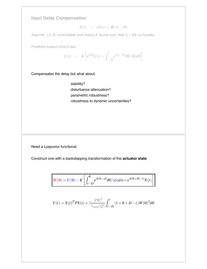
Input Delay Compensation ˙ X ( t ) = AX ( t )+ BU ( t − D ) Assume: ( A , B ) controllable and matrix K found such that A + BK is Hurwitz. Predictor-based control law: Z t � � e AD X ( t )+ t − D e A ( t − θ ) BU ( θ ) d θ U ( t ) = K Compensates the delay but what about: stability? disturbance attenuation? parametric robustness? robustness to dynamic uncertainties? Need a Lyapunov functional. Construct one with a backstepping transformation of the actuator state : � Z θ � t − D e A ( θ − σ ) BU ( σ ) d σ + e A ( θ + D − t ) X ( t ) W ( θ ) = U ( θ ) − K Z t V ( t ) = X ( t ) T PX ( t )+ 2 | PB | 2 t − D ( 1 + θ + D − t ) W ( θ ) 2 d θ λ min ( Q )

Is there any benefit to having a Lyapunov function besides proving stability? Inverse optimality and robustness to actuator lag. Theorem 1 There exists c ∗ such that the feedback system with the controller Z t � � �� c e AD X ( t )+ t − D e A ( t − θ ) BU ( θ ) d θ U ( t ) = K , s + c is exponentially stable in the sense of the norm Z t � � 1 / 2 | X ( t ) | 2 + t − D U ( θ ) 2 d θ + U ( t ) 2 N ( t ) = for all c > c ∗ . Furthermore, there exists c ∗∗ > c ∗ such that, for any c ≥ c ∗∗ , the feedback minimizes the cost functional Z ∞ � U ( t ) 2 � Q ( t )+ ˙ J = dt , 0 where Q ( t ) ≥ µN ( t ) 2 for some µ ( c ) > 0 , which is such that µ ( c ) → ∞ as c → ∞ . With a Lyapunov function, one can even quantify disturbance attenuation ˙ X ( t ) = AX ( t )+ BU ( t − D )+ Gd ( t ) Theorem 2 ∃ c ∗ s.t. ∀ c > c ∗ , the feedback system is L ∞ -stable, i.e., ∃ positive constants β 1 , β 2 , γ 1 s.t. N ( t ) ≤ β 1 e − β 2 t N ( 0 )+ γ 1 sup | d ( τ ) | . τ ∈ [ 0 , t ] Furthermore, ∃ c ∗∗ > c ∗ s.t. ∀ c ≥ c ∗∗ the feedback minimizes the cost functional Z t � � � U ( t ) 2 − c γ 2 d ( τ ) 2 � Q ( τ )+ ˙ J = sup lim 2 cV ( t )+ d τ t → ∞ 0 d ∈ D for any 2 = 8 λ max ( PBB T P ) γ 2 ≥ γ ∗∗ , λ min ( Q ) where Q ( t ) ≥ µN ( t ) 2 for some µ ( c , γ 2 ) > 0 , which is such that µ ( c , γ 2 ) → ∞ as c → ∞ , and D is the set of linear scalar-valued functions of X .

Robustness to Delay Mismatch The biggest open question in robustness of predictor feedbacks. ˙ X = AX + BU ( t − D 0 − Δ D ) Z t � � e AD 0 X ( t )+ e A ( t − θ ) BU ( θ ) d θ U ( t ) = K t − D 0 Δ D either positive or negative Theorem 3 ∃ δ > 0 s.t. ∀ Δ D ∈ ( − δ , δ ) the closed-loop system is exp. stable in the sense of the state norm Z t � � 1 / 2 | X ( t ) | 2 + D U ( θ ) 2 d θ N 2 ( t ) = , t − where D = D 0 + max { 0 , Δ D } . Corollary 1 ∃ δ > 0 s.t. ∀ D 0 ∈ [ 0 , δ ) the system ˙ X = AX + BU ( t ) , Z t � � e AD 0 X ( t )+ e A ( t − θ ) BU ( θ ) d θ U ( t ) = K t − D 0 � � 1 / 2 R t | X ( t ) | 2 + t − D 0 U ( θ ) 2 d θ is exp. stable in the sense of the norm .

Delay-Robustness of Predictor Feedback LTI-ODE U ( t ) uncertain delay plant Delay-Adaptive Control LTI-ODE U ( t ) uncertain delay plant LTI-ODE U ( t ) unknown delay plant Motivation: control of thermoacoustic instabilities in gas turbine combustors

transport PDE with certainty equivalence U ( t ) X ( t ) LTI-ODE version of unknown plant propagation speed 1/ D predictor feedback u ( x , t ) estimator of D Update law reg. regressor error Z 1 � �� � � �� � K e A ˆ D ( t ) x dx ( AX ( t )+ Bu ( 0 , t )) 0 ( 1 + x ) w ( x , t ) d ˆ D ( t ) = − γ Z 1 dt 1 + X ( t ) T PX ( t )+ b 0 ( 1 + x ) w ( x , t ) 2 dx � �� � normalization Z x 0 K e A ˆ D ( t )( x − y ) Bu ( y , t ) dy − K e A ˆ D ( t ) x X ( t ) . u ( x , t ) − ˆ w ( x , t ) = D ( t )

Update law reg. regressor error Z 1 � �� � � �� � K e A ˆ D ( t ) x dx ( AX ( t )+ Bu ( 0 , t )) 0 ( 1 + x ) w ( x , t ) d ˆ D ( t ) = − γ Z 1 dt 1 + X ( t ) T PX ( t )+ b 0 ( 1 + x ) w ( x , t ) 2 dx � �� � normalization Z x 0 K e A ˆ D ( t )( x − y ) Bu ( y , t ) dy − K e A ˆ D ( t ) x X ( t ) . u ( x , t ) − ˆ w ( x , t ) = D ( t ) ∃ R , ρ > 0 s.t. Theorem 4 � � � � ϒ ( t ) ≤ R exp ρϒ ( 0 ) − 1 (exp. growing class K ∞ glob. stab. bound) where Z 1 � 2 . ϒ ( t ) = | X ( t ) | 2 + � 0 u ( x , t ) 2 dx + D − ˆ D ( t ) X ( t ) , U ( t ) → 0 . Furthermore, 1.4 ^ 2 D (0) = 2 ^ D (0) = 2 ^ D (0) = 0 ^ D (0) = 0 1.2 1.5 1 0.8 D(t) X ( t ) ^ 1 0.6 0.4 0.5 0.2 0 0 0 2 4 6 8 10 0 2 4 6 8 10 t t 0.5 0 e − s − 0.5 X ( s ) = s − 0 . 75 U ( s ) U ( t ) − 1 − 1.5 ^ D (0) = 2 ^ D (0) = 0 Simulations by − 2 Delphine Bresch-Pietri − 2.5 0 2 4 6 8 10 t

0–1 sec The delay precludes any influence of the control on the plant, so X ( t ) shows an exponential open-loop growth. 1–3 sec The plant starts responding to the control and its evolution changes qualitatively, resulting also in a qualitative change of the control signal. 3–4 sec When the estimation of ˆ D ( t ) ends at about 3 seconds, the controller structure becomes linear. However, due to the delay, the plant state X ( t ) continues to evolve based on the inputs from 1 second earlier, so, a non-monotonic transient continues until about 4 seconds. 4 sec and onwards The ( X , U ) system is linear and the delay is sufficiently well compen- sated, so the response of X ( t ) and U ( t ) shows a monotonically decaying exponential trend of a first order system. Time-Varying Input Delay Basic idea introduced by Artstein (TAC, 1982) , but only conceptually (nor explicitly), for LT V systems with TV delays. Explicit design for LTI plants presented by Nihtila (CDC, 1991) , but no analysis of stability or of feasibility of the controller.

Time-Varying Input Delay ˙ X ( t ) = AX ( t )+ BU ( φ ( t )) φ ( t ) = t − D ( t ) : = “delayed time” Predictor feedback Z t � � � � � � φ − 1 ( t ) − t φ − 1 ( t ) − φ − 1 ( θ ) U ( θ ) e A φ ( t ) e A U ( t ) = K X ( t )+ B � d θ φ ′ � φ − 1 ( θ ) Time-Varying Delay ˙ X ( t ) = AX ( t )+ BU ( φ ( t )) Predictor feedback Z t � � � � � � φ − 1 ( t ) − t φ − 1 ( t ) − φ − 1 ( θ ) U ( θ ) e A φ ( t ) e A U ( t ) = K X ( t )+ B � d θ φ − 1 ( θ ) φ ′ � Transport PDE representation � � � ��� φ − 1 ( t ) − t u ( x , t ) = U t + x φ Time-varying backstepping transformation Z x � � � � φ − 1 ( t ) − t φ − 1 ( t ) − t w ( x , t ) = u ( x , t ) − K e Ax 0 e A ( x − y ) � � φ − 1 ( t ) − t X ( t ) − K Bu ( y , t ) dy

Need a Lyapunov functional. Construct one with a backstepping transformation of the actuator state : X ( φ − 1 ( θ ) � P ( θ ) � �� � � � � � Z θ � � φ − 1 ( θ ) − t φ − 1 ( θ ) − φ − 1 ( σ ) U ( σ ) e A φ ( t ) e A W ( θ ) = U ( θ ) − K X ( t )+ B � d σ φ ′ � φ − 1 ( σ ) φ ( t ) ≤ θ ≤ t Need a Lyapunov functional. Construct one with a backstepping transformation of the actuator state : X ( φ − 1 ( θ ) � P ( θ ) � �� � � � � � Z θ � � φ − 1 ( θ ) − t φ − 1 ( θ ) − φ − 1 ( σ ) U ( σ ) e A φ ( t ) e A W ( θ ) = U ( θ ) − K X ( t )+ B � d σ φ ′ � φ − 1 ( σ ) φ ( t ) ≤ θ ≤ t b φ − 1 ( θ ) − t Z t φ − 1 ( t ) − t e V ( t ) = X ( t ) T PX ( t )+ a � W ( θ ) 2 d θ � � φ ′ � φ − 1 ( t ) − t φ − 1 ( θ ) φ ( t )

Theorem 1 ∃ G , g > 0 s.t. Z t Z 0 � � | X ( t ) | 2 + | X 0 | 2 + t − D ( t ) U 2 ( θ ) d θ ≤ G e − gt − D ( 0 ) U 2 ( θ ) d θ , ∀ t ≥ 0 , where G (but not g ) depends on the function D ( · ) . Target system ˙ X ( t ) = ( A + BK ) X ( t )+ Bw ( 0 , t ) , w t ( x , t ) = π ( x , t ) w x ( x , t ) , w ( 1 , t ) = 0 , where the variable speed of propagation is   � � φ − 1 ( t ) d  1 + x − 1   dt  π ( x , t ) = φ − 1 ( t ) − t Theorem 5 Let the delay function δ ( t ) = t − φ ( t ) be strictly positive and uniformly bounded Let the delay rate function δ ′ ( t ) be strictly smaller than 1 and uniformly from above. bounded from below. There exist positive constants G and g (the latter one being in- dependent of φ ) such that Z t Z 0 � � | X ( t ) | 2 + | X 0 | 2 + φ ( t ) U 2 ( θ ) d θ ≤ G e − gt φ ( 0 ) U 2 ( θ ) d θ , for all t ≥ 0 .

Nonlinear systems with constant delay Nonlinear Systems with Constant Input Delay ˙ X ( t ) = f ( X ( t ) , U ( t − D )) Assumptions: ˙ X = f ( X , κ ( X )) is g.a.s. ˙ X = f ( X , U ) is forward complete Predictor-based controller (predictor given implicitly in general): U ( t ) = κ ( P ( t )) Z t P ( t ) = X ( t )+ t − D f ( P ( θ ) , U ( θ )) d θ

Nonlinear stabilization when delay is a function of state Miroslav Krstic Sontagfest , May 2011 Conditions on the delay function D ( t ) = t − φ ( t ) : • D ( t ) ≥ 0 (causality); • D ( t ) is uniformly bounded from above (all inputs applied to the plant eventually reach the plant); • D ′ ( t ) < 1 (plant never feels input values that are older than the ones it has already felt— input signal direction never reversed ); • D ′ ( t ) is uniformly bounded from below (delay cannot disappear instantaneously, but only gradually).