
SLIDE 1
Image and Video Coding: Motion Estimation and Coding
A C D0 D1 B E0 E1
current block
1 2 3 4 5 6 7
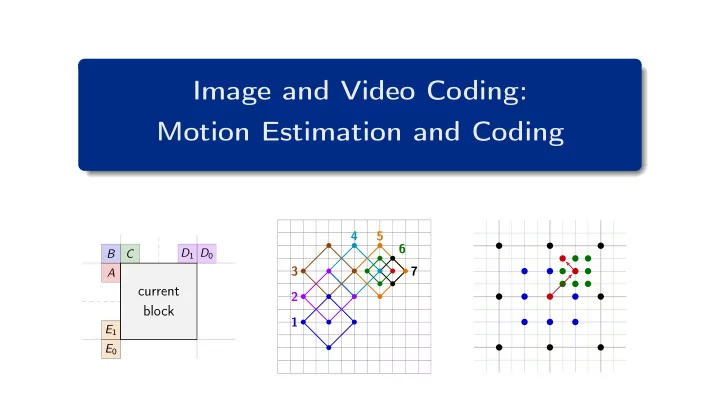
Image and Video Coding: Motion Estimation and Coding 4 5 6 B C - - PowerPoint PPT Presentation
Image and Video Coding: Motion Estimation and Coding 4 5 6 B C D 1 D 0 3 7 A current 2 block 1 E 1 E 0 Last Lecture Last Lecture: Hybrid Video Coding Hybrid Video Coding Partitioning of pictures into blocks current picture
A C D0 D1 B E0 E1
1 2 3 4 5 6 7
Last Lecture
ref[ x + mx, y + my ]
x y displacement vector for current block m = (mx, my) current picture displaced object best matching block in reference picture reconstructed reference picture moving object
Heiko Schwarz (Freie Universität Berlin) — Image and Video Coding: Motion Estimation and Coding 2 / 38
Picture Partitioning / Variable Block Sizes
Heiko Schwarz (Freie Universität Berlin) — Image and Video Coding: Motion Estimation and Coding 3 / 38
Picture Partitioning / Variable Block Sizes
Heiko Schwarz (Freie Universität Berlin) — Image and Video Coding: Motion Estimation and Coding 4 / 38
Picture Partitioning / Variable Block Sizes
root
1 1 1 1 1 1
Heiko Schwarz (Freie Universität Berlin) — Image and Video Coding: Motion Estimation and Coding 5 / 38
Picture Partitioning / Variable Block Sizes
luma and chroma interpolation filters of HEVC phase
1 2 3 4 1/4
4
58 17
1 luma 1/2
4
40 40
4
3/4 1
17 58
4
1/8
58 10
1/4
54 16
3/8
46 28
chroma 1/2
36 36
5/8
28 46
3/4
16 54
7/8
10 58
Heiko Schwarz (Freie Universität Berlin) — Image and Video Coding: Motion Estimation and Coding 6 / 38
Picture Partitioning / Supported Block Sizes in Video Coding Standards
1 One motion vector per macroblock 2 Macroblock is split into four 8×8 blocks,
Heiko Schwarz (Freie Universität Berlin) — Image and Video Coding: Motion Estimation and Coding 7 / 38
Picture Partitioning / Supported Block Sizes in Video Coding Standards
1 Four modes for partitioning into sub-macroblocks Inter-16x16, Inter-16x8, Inter-8x16, Inter-8x8 2 8×8 sub-macroblocks can be further subdivided 8x8, 8x4, 4x8, 4x4
1 Four 8×8 transform blocks not allowed if motion blocks smaller 8×8 are used 2 Sixteen 4×4 transform blocks
Inter-16x16 Inter-16x8 Inter-8x16 Inter-8x8 8x8 8x4 4x8 4x4 luma 8x8 luma 4x4 chroma
Heiko Schwarz (Freie Universität Berlin) — Image and Video Coding: Motion Estimation and Coding 8 / 38
Picture Partitioning / Supported Block Sizes in Video Coding Standards
1 Initial partitioning into Coding Tree Units (CTUs)
2 Quadtree partitioning into Coding Units (CUs)
CTU
N > 8, N = Nmin
N×N N×(N/2) (N/2)×N (N/2)×(N/2)
N > 8
N×(N/4) N×(3N/4) (N/4)×N (3N/4)×N Heiko Schwarz (Freie Universität Berlin) — Image and Video Coding: Motion Estimation and Coding 9 / 38
Picture Partitioning / Supported Block Sizes in Video Coding Standards
1 4 1 2 1 4
Th
1/4 1/2 1/4
Tv
1/2 1/2
Bh
1/2 1/2
Bv no
1/2 1/2
Q
split codeword no Q 1 1 Bh 1 0 0 1 Bv 1 0 1 1 Th 1 0 0 0 Tc 1 0 1 0 CTU
Q Bh Tv Q Bv Bv Tv Th Bh Q Th Bh no no no no Heiko Schwarz (Freie Universität Berlin) — Image and Video Coding: Motion Estimation and Coding 10 / 38
Picture Partitioning / Coding Order and Encoder Decision
1 From top to bottom 2 From left to right
Heiko Schwarz (Freie Universität Berlin) — Image and Video Coding: Motion Estimation and Coding 11 / 38
Picture Partitioning / Coding Order and Encoder Decision
example: two-level quadtree 1 2 3 4 5
Heiko Schwarz (Freie Universität Berlin) — Image and Video Coding: Motion Estimation and Coding 12 / 38
Picture Partitioning / Coding Order and Encoder Decision
example: two-level quadtree 1 2 4 6 7 3 5
Heiko Schwarz (Freie Universität Berlin) — Image and Video Coding: Motion Estimation and Coding 13 / 38
Picture Partitioning / Coding Efficiency
30 31 32 33 34 35 36 37 38 39 5 10 15 20 25 30 4×4 8×8 16×16 32×32 64×64 adaptive PSNR (Y) [dB] bit rate [Mbit/s] Cactus (1920×1080, 50 Hz) IPPP, 4×4 transform bit-rate saving of adaptive vs 16×16: 23 % on average 35 36 37 38 39 40 41 42 43 44 1 2 3 4 5 4×4 8×8 16×16 32×32 64×64 adaptive PSNR (Y) [dB] bit rate [Mbit/s] Johnny (1280×720, 60 Hz) IPPP, 4×4 transform bit-rate saving of adaptive vs 32×32: 35 % on average
Heiko Schwarz (Freie Universität Berlin) — Image and Video Coding: Motion Estimation and Coding 14 / 38
Picture Partitioning / Coding Efficiency
30 31 32 33 34 35 36 37 38 39 5 10 15 20 25 30 4×4 8×8 16×16 32×32 64×64 adaptive PSNR (Y) [dB] bit rate [Mbit/s] Cactus (1920×1080, 50 Hz) IPPP, all transform sizes bit-rate saving of adaptive vs 16×16: 22 % on average 35 36 37 38 39 40 41 42 43 44 1 2 3 4 5 4×4 8×8 16×16 32×32 64×64 adaptive PSNR (Y) [dB] bit rate [Mbit/s] Johnny (1280×720, 60 Hz) IPPP, all transform sizes bit-rate saving of adaptive vs 32×32: 29 % on average
Heiko Schwarz (Freie Universität Berlin) — Image and Video Coding: Motion Estimation and Coding 15 / 38
Picture Partitioning / Coding Efficiency
impact of supported block sizes bit-rate savings relative to ... MPEG-2 H.263 H.264 H.265 H.263 4 % H.264/AVC 9 % 5 % H.265/HEVC 35 % 32 % 28 % H.266/VVC 40 % 37 % 34 % 9 %
Heiko Schwarz (Freie Universität Berlin) — Image and Video Coding: Motion Estimation and Coding 16 / 38
Coding of Motion Parameters
Heiko Schwarz (Freie Universität Berlin) — Image and Video Coding: Motion Estimation and Coding 17 / 38
Coding of Motion Parameters / Motion Vector Prediction
MVD coding in HEVC ∆m codeword ±1 10s ±2 1110 s ±3 1111 s ±4 1101 00s ±5 1101 01s ±6 1101 10s ±7 1101 11s ±8 1100 1000 s ±9 1100 1001 s ±10 1100 1010 s ±11 1100 1011 s ±12 1100 1100 s ±13 1100 1101 s ±14 1100 1110 s ±15 1100 1111 s ±16 1100 0100 00s ±17 1100 0100 01s · · · · · ·
Heiko Schwarz (Freie Universität Berlin) — Image and Video Coding: Motion Estimation and Coding 18 / 38
Coding of Motion Parameters / Motion Vector Prediction
x ,
y
x , mB x , mC x
y , mB y , mC y
Heiko Schwarz (Freie Universität Berlin) — Image and Video Coding: Motion Estimation and Coding 19 / 38
Coding of Motion Parameters / Motion Vector Prediction
A0 A1 B0 B1 B2
T0 T1 co-located area in reference picture
Heiko Schwarz (Freie Universität Berlin) — Image and Video Coding: Motion Estimation and Coding 20 / 38
Coding of Motion Parameters / Modes with Inferred Motion Parameters
time
co-located block current block
Heiko Schwarz (Freie Universität Berlin) — Image and Video Coding: Motion Estimation and Coding 21 / 38
Coding of Motion Parameters / Modes with Inferred Motion Parameters
A0 A1 B0 B1 B2
T0 T1 co-located area in reference picture
Heiko Schwarz (Freie Universität Berlin) — Image and Video Coding: Motion Estimation and Coding 22 / 38
Coding of Motion Parameters / Modes with Inferred Motion Parameters
A
∆m0 ∆m1 = −∆m0
Heiko Schwarz (Freie Universität Berlin) — Image and Video Coding: Motion Estimation and Coding 23 / 38
Estimation of Motion Vectors / Cost Measure for Motion Search
ref[x + mx, y + my]
ref[ x, y ]
current original picture s[ x, y ]
Heiko Schwarz (Freie Universität Berlin) — Image and Video Coding: Motion Estimation and Coding 24 / 38
Estimation of Motion Vectors / Cost Measure for Motion Search
m∈R D(m) + λm · R(m)
Hadamard Transform Defined for integer powers of 2 A1 =
1 √ 2
AN/2 AN/2 −AN/2
A4 = 1 2 1 1 1 1 1 −1 1 −1 1 1 −1 −1 1 −1 −1 1 Hadamard SAD
1 Calculate Hadamard Transform of
prediction error s[x, y] − ˆ s[x, y]
2 Sum up absolute values of the
Hadamard transform coefficients
Heiko Schwarz (Freie Universität Berlin) — Image and Video Coding: Motion Estimation and Coding 25 / 38
Estimation of Motion Vectors / Cost Measure for Motion Search
5 10 15 20 25 30 35 40 36 37 38 39 40 41 42 43 44 Full transform coding (avg. 17.8 %) SSD (avg. 6.5 %) SAD (avg. 6.6 %) Hadamard SAD (avg. 12.2 %) bit-rate saving vs SAD-based ME [%] PSNR (Y) [dB] Kimono (1920×1080, 24 Hz)
Heiko Schwarz (Freie Universität Berlin) — Image and Video Coding: Motion Estimation and Coding 26 / 38
Estimation of Motion Vectors / Sub-Sample Refinement
1 Integer sample search 2 Sub-sample refinement(s)
integer-sample locations tested half-sample locations tested quarter-sample locations
Heiko Schwarz (Freie Universität Berlin) — Image and Video Coding: Motion Estimation and Coding 27 / 38
Estimation of Motion Vectors / Sub-Sample Refinement
5 10 15 20 25 30 35 40 36 37 38 39 40 41 42 43 44 Exhaustive Search: Hadamard SAD (avg. 12.2 %) Refinement: HSAD + HSAD (avg. 10.3 %) Refinement: SAD + HSAD (avg. 9.3 %) Refinement: SAD + SAD (avg. 5.3 %) bit-rate saving vs TM5-ME [%] PSNR (Y) [dB] Kimono (1920×1080, 24 Hz)
Heiko Schwarz (Freie Universität Berlin) — Image and Video Coding: Motion Estimation and Coding 28 / 38
Estimation of Motion Vectors / Fast Integer Search Strategies
[ Jain, Jain, 1981 ]
Heiko Schwarz (Freie Universität Berlin) — Image and Video Coding: Motion Estimation and Coding 29 / 38
Estimation of Motion Vectors / Fast Integer Search Strategies
[ Li, Zeng, Liou, 1994 ]
Heiko Schwarz (Freie Universität Berlin) — Image and Video Coding: Motion Estimation and Coding 30 / 38
Estimation of Motion Vectors / Fast Integer Search Strategies
A C D0 D1 B E0 E1
Heiko Schwarz (Freie Universität Berlin) — Image and Video Coding: Motion Estimation and Coding 31 / 38
Estimation of Motion Vectors / Fast Integer Search Strategies
5 10 15 20 25 30 35 40 36 37 38 39 40 41 42 43 44 Exhaustive integer search (avg. 9.3 %) Fast integer search (avg. 9.1 %) bit-rate saving vs SAD-based ME [%] PSNR (Y) [dB] Kimono (1920×1080, 24 Hz)
Heiko Schwarz (Freie Universität Berlin) — Image and Video Coding: Motion Estimation and Coding 32 / 38
Increased Flexibility of Motion Description / Motion Vectors Outside Picture Boundaries
reference picture current picture
Heiko Schwarz (Freie Universität Berlin) — Image and Video Coding: Motion Estimation and Coding 33 / 38
Increased Flexibility of Motion Description / Higher Order Motion Models
4 parameter model affine model
Heiko Schwarz (Freie Universität Berlin) — Image and Video Coding: Motion Estimation and Coding 34 / 38
Increased Flexibility of Motion Description / Higher Order Motion Models
perspective model parabolic model
Heiko Schwarz (Freie Universität Berlin) — Image and Video Coding: Motion Estimation and Coding 35 / 38
Increased Flexibility of Motion Description / Higher Order Motion Models
ref
Heiko Schwarz (Freie Universität Berlin) — Image and Video Coding: Motion Estimation and Coding 36 / 38
Increased Flexibility of Motion Description / Higher Order Motion Models
6-parameter model: 3 control point motion vectors 4-parameter model: 2 control point motion vectors
Heiko Schwarz (Freie Universität Berlin) — Image and Video Coding: Motion Estimation and Coding 37 / 38
Summary
Heiko Schwarz (Freie Universität Berlin) — Image and Video Coding: Motion Estimation and Coding 38 / 38