
SLIDE 1
10/8/2019 1
2
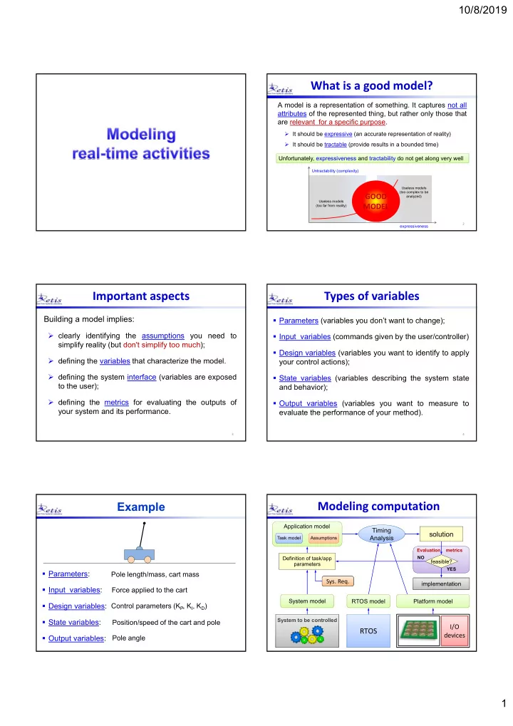
What is a good model?
- It should be expressive (an accurate representation of reality)
- It should be tractable (provide results in a bounded time)
Unfortunately, expressiveness and tractability do not get along very well Unfortunately, expressiveness and tractability do not get along very well
expressiveness Untractability (complexity)
Useless models (too far from reality) Useless models (too complex to be analyzed)
GOOD MODEL
A model is a representation of something. It captures not all attributes of the represented thing, but rather only those that are relevant for a specific purpose.
3
Important aspects
Building a model implies:
- clearly identifying the assumptions you need to
simplify reality (but don't simplify too much);
- defining the variables that characterize the model.
- defining the system interface (variables are exposed
to the user);
- defining the metrics for evaluating the outputs of
your system and its performance.
4
Types of variables
- Parameters (variables you don’t want to change);
- Input variables (commands given by the user/controller)
- Design variables (variables you want to identify to apply
your control actions);
- State variables (variables describing the system state
and behavior);
- Output variables (variables you want to measure to
evaluate the performance of your method).
Example
- Parameters:
- Input variables:
- Design variables:
- State variables:
- Output variables:
Pole length/mass, cart mass Force applied to the cart Control parameters (KP, KI, KD) Position/speed of the cart and pole Pole angle
Application model
6
Modeling computation
Task model Task model
System to be controlled Definition of task/app parameters
- Sys. Req.
- Sys. Req.
I/O devices I/O devices
RTOS RTOS
Timing Analysis Timing Analysis
solution
System model System model Platform model Platform model RTOS model RTOS model
Assumptions Assumptions
implementation implementation
feasible?
NO YES Evaluation metrics