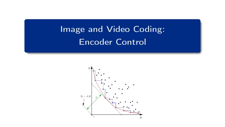
Image and Video Coding: Encoder Control D D = - R d R Problem - - PowerPoint PPT Presentation

Image and Video Coding: Encoder Control

D = -λ R d

D R

Problem Statement / Scope of Image and Video Coding Standards

Image and Video Coding

scope of standards

pre- processing image/video encoder image/video decoder post- processing

input samples bitstream

• utput

samples

Interoperability and Standards Bitstream generated by an encoder should be reliably decodable by decoders of other manufacturers Image and video coding standards define “interface” between encoder and decoder Scope of Image and Video Coding Standards

1 Bitstream syntax

(including constraints for transmitted and derived parameters)

2 Decoding process

(example decoding process for conforming bitstreams) No guarantee of image/video quality Coding efficiency is determined by all components

Heiko Schwarz (Freie Universität Berlin) — Image and Video Coding: Encoder Control 2 / 35

Problem Statement / Coding Efficiency

Coding Efficiency: Trade-Off between Bit Rate and Reconstruction Quality

Bit Rate Use average bit rate in our comparisons (count bits in bitstream) R =

number of bits in bitstream for the video sequence nominal duration of the video sequence (in seconds)

• in bits/s
• Reconstruction Quality

Human perception of visual quality: Difficult to evaluate (subjective tests) Use mean squared error (MSE) and peak signal-to-noise ratio (PSNR) MSE = 1 W · H

• ∀x,y
• s′[x, y] − s[x, y]

2 PSNR [dB] = 10 · log10 s2

max

MSE

• maximum sample value: smax = 2B − 1
• Heiko Schwarz (Freie Universität Berlin)

— Image and Video Coding: Encoder Control 3 / 35

Problem Statement / Coding Efficiency

Coding Efficiency: Rate-Distortion Curves & Bit-Rate Savings

35 36 37 38 39 40 41 1000 2000 3000 4000 5000 codec B codec A RB RA example target quality ( 39 dB ) PSNR [dB] bit rate [kbit/s] 10 20 30 40 50 60 70 36 37 38 39 40 41 BBA = (RA - RB) / RA target quality ( 39 dB ) example bit rate saving of codec B vs. codec A bit-rate saving [%] PSNR [dB]

Rate-Distortion Curve Measure average bit rate and average PSNR for multiple operation points Bit-Rate Savings Determine bit-rate savings using interpolated rate-distortion curves BBA = (RA − RB)/RA

• codec B relative to codec A
• Average bit-rate savings: Can be calculated by integrating curve

Heiko Schwarz (Freie Universität Berlin) — Image and Video Coding: Encoder Control 4 / 35

Problem Statement / Impact of Encoder Control

Coding Efficiency of Image and Video Codecs

syntax & decoding process

image/video encoder image/video decoder

• riginal

samples bitstream reconstructed samples

Bitstream Syntax and Decoding Process Specify syntax features and supported coding tools Determine maximum achievable coding efficiency Image/Video Encoder Lot of freedom to choose coding parameters (modes, motion vectors, quantization indexes, ...) Encoding process determines coding efficiency of a bitstream for given syntax and decoder Main Encoding Problem Select coding parameters such that the coding efficiency is maximized

Heiko Schwarz (Freie Universität Berlin) — Image and Video Coding: Encoder Control 5 / 35

Problem Statement / Impact of Encoder Control

Example: Which Quantization Method is Better ?

• abs. transform coeffs. |uk|

93 46 24 4 2 1 3 4 37 4 4 3 1 2 6 14 4 2 3 2 3 3 1 7 3 1 3 1 2 3 1 2 1 4 3 2 4 2 1 2 1 1 3 1 1 1 2 2 1 2 1 2 1 3 1 excerpt of MPEG-2 table (run, level) codeword (s = sign) (eob) 10 (0, ±1) 11s (0, ±4) 0000 110s (0, ±5) 0010 0110 s (0, ±9) 0000 0001 1101 s (1, ±2) 0001 10s (3, ±1) 0011 1s (escape) 0000 01 (+18 bits) note: there is no (32, ±1) pair

simple rounding: qk = round uk ∆

• quantization step size

∆ = 10

• abs. quant. indexes |qk|

9 5 2 0 4 0 0 1 0 1 0 0 0 0 0 0 0 0 1 0 0 0 0 0 0 0 0 0 0 0 0 0 0 0 0 0 0 0 0 0 0 0 0 0 0 0 0 0 0 0 0 0 0 0 0 0 0 0 0 0 0 0 0

run-level pairs (absolute levels): (0,9) (0,5) (0,4) (0,1) (1,2) (3,1) (32,1) (eob) distortion (SSD): D1 =

• ∀k

(uk − ∆·qk)2 = 371 number of bits: R1 = 13 + 9 + 8 + 3 + 7 + 6 + 24 + 2 R1 = 72 bits run-level pairs (absolute levels): (0,9) (0,5) (0,4) (0,1) (1,2) (3,1) (eob) distortion (SSD): D2 =

• ∀k

(uk − ∆·qk)2 = 391 (- 0.23 dB) number of bits: R1 = 13 + 9 + 8 + 3 + 7 + 6 + 2 R2 = 48 bits (- 33.3 %)

alternative quantization method

quantization step size

∆ = 10

• abs. quant. indexes |qk|

9 5 2 0 4 0 0 1 0 1 0 0 0 0 0 0 0 0 0 0 0 0 0 0 0 0 0 0 0 0 0 0 0 0 0 0 0 0 0 0 0 0 0 0 0 0 0 0 0 0 0 0 0 0 0 0 0 0 0 0 0 0 0 0

Heiko Schwarz (Freie Universität Berlin) — Image and Video Coding: Encoder Control 6 / 35

Problem Statement / Impact of Encoder Control

Quantization Example: Impact on Coding Efficiency simple quantization alternative quantization method same quantization step size ∆ bit rate PSNR

Heiko Schwarz (Freie Universität Berlin) — Image and Video Coding: Encoder Control 7 / 35

Problem Statement / Impact of Encoder Control

Example: Motion Estimation and Mode Decision

Motion Estimation Goal: Find matching block in reference picture Match with minimum distortion: SSD distortion: D = 273 motion vector: m = (30, 38) 22 bits (EG0) Alternative match: SSD distortion: D = 295 (−0.34 dB) motion vector: m = (2, −1) 8 bits (-64 %) Mode Decision How to decide between intra and inter coding for a block? How to decide between different coding modes?

reconstructed reference picture current picture

Heiko Schwarz (Freie Universität Berlin) — Image and Video Coding: Encoder Control 8 / 35

Lagrangian Encoder Control / Encoding Problem

General Encoding Problem in Image and Video Coding

Given Bitstream syntax (format for transmitting coding parameters) Decoding process (algorithm for reconstructing pictures) Encoding Problem Choose coding parameters (and thus the bistream) in a way that coding efficiency is maximized Selection of coding modes Selection of motion parameters Selection of quantization indexes Criterion for Coding Efficiency Need to consider both Quality (or distortion) of reconstructed pictures Bit rate of resulting bitstream

Heiko Schwarz (Freie Universität Berlin) — Image and Video Coding: Encoder Control 9 / 35

Lagrangian Encoder Control / Encoding Problem

Encoding Problem: Mathematically Formulation

Formulation of Encoding Problem Find conforming bitstream b∗ that minimizes the distortion D for the given input image/video sv and has a bit rate R that does not exceed a bit rate budget RB b∗ = arg min

∀ b∈B

D

• sv, s′

v(b)

• subject to

R(b) ≤ RB with

sv : samples of entire image/video s′

v(b) :

reconstructed image/video for bitstream b D(sv, s′

v) :

distortion between original and reconstructed image/video B : set of all conforming bitstreams RB : maximum available bit rate for encoding task

Impossible to find optimal solution (extremely large parameter space) Split into smaller sub-problems

Heiko Schwarz (Freie Universität Berlin) — Image and Video Coding: Encoder Control 10 / 35

Lagrangian Encoder Control / Lagrangian Optimization

Lagrangian Optimization for Discrete Sets

Constrained Optimization Problem Consider set of samples s (block, picture) and discrete vector of coding parameters p Constrained problem for given rate budget RB, with D(p) = D

• s, s′(p)
• popt(RB) = arg min

p

D(p) subject to R(p) ≤ RB Varying RB: Optimal coding parameter vectors {popt} Unconstrained Optimization Problem Using Lagrange multipliers λ ≥ 0, we obtain the unconstrained problem p∗

λ = arg min p

D(p) + λ · R(p) Cannot find all optimal solutions {popt} But: Each solution p∗

λ is an optimal solution, {p∗ λ} ⊆ {popt}

Heiko Schwarz (Freie Universität Berlin) — Image and Video Coding: Encoder Control 11 / 35

Lagrangian Encoder Control / Lagrangian Optimization

Optimality of Lagrangian Approach

Consider solution p∗

λ for a particular value of λ, with λ ≥ 0

By definition, we have ∀p, D(p) + λ · R(p) ≥ D(p∗

λ) + λ · R(p∗ λ)

D(p) − D(p∗

λ) ≥ λ ·

• R(p∗

λ) − R(p)

• Since λ ≥ 0, the above inequality implies

∀p : R(p) ≤ R(p∗

λ),

D(p) ≥ D(p∗

λ)

Hence, p∗

λ is a solution of the constrained problem

p∗

λ = arg min p

D(p) subject to R(p) ≤ RB = R(p∗

λ)

Each solution of the unconstrained optimization problem is also a solution of original constrained optimization problem

Heiko Schwarz (Freie Universität Berlin) — Image and Video Coding: Encoder Control 12 / 35

Lagrangian Encoder Control / Lagrangian Optimization

Illustration of Lagrangian Optimization

RB

D = -λ R d solution of constrained problem solution of unconstrained problem convex hull tangent with slope -λ

D R

d (1+λ2)0.5 solution of unconstrained problem convex hull tangent parallel to R-axis

D+λR R

Solutions of Lagrangian optimization problem minimize distance d to lines D = −λ · R Subset {p∗

λ} lies on convex hull of area of all possible rate-distortion points

Heiko Schwarz (Freie Universität Berlin) — Image and Video Coding: Encoder Control 13 / 35

Lagrangian Encoder Control / Lagrangian Bit Allocation

Lagrangian Bit Allocation

Lagrangian Optimization for Independent Subsets Consider partitioning of s into independent subsets sk (for example: picture into blocks) Consider any additive distortion measure, D = Dk Overall optimization problem {p∗

0, p∗ 1, · · · } = arg

min

p0,p1,···

• ∀k

Dk(pk) + λ

• ∀k

Rk(pk) Can be solved by separate minimizations (with same Lagrange multiplier λ ) ∀k, p∗

k = min pk

Dk(pk) + λ Rk(pk) Key Advantage of Lagrangian Optimization Global optimization problem can be solved by separate minimizations Yields optimal bit allocation {R0, R1, · · · }

Heiko Schwarz (Freie Universität Berlin) — Image and Video Coding: Encoder Control 14 / 35

Lagrangian Encoder Control / Lagrangian Bit Allocation

Illustration of Lagrangian Bit Allocation

D R subset A subset B subset C subset D subset E convex hull D R not optimal

• ptimal, not on convex hull
• ptimal, on convex hull

Example: 5 subsets (A,B,C,D,E), each with 6 operating points Options for entire set: 65 = 7776 coding options Constrained optimization: Evaluate all 7776 combinations Lagrangian approach: Only 30 comparisons required (6 per subset)

Heiko Schwarz (Freie Universität Berlin) — Image and Video Coding: Encoder Control 15 / 35

Lagrangian Encoder Control / Lagrangian Bit Allocation

Lagrangian Optimization for Non-Independent Sets

In Practice: Decisions for blocks are not independent of each other Motion-compensated prediction Intra-picture prediction Predictive and conditional entropy coding (e.g., run-level coding) Concept of Lagrangian Optimization is Still Applicable Partly neglect dependencies between coding decisions Approach with same complexity as the method for independent sets p∗

k = arg min pk

Dk(pk | pk−1, pk−2, · · · ) + λ · Rk(pk | pk−1, pk−2, · · · ) Past decisions {pk−1, pk−2, · · · } are taken into account (by using correct predictors and conditional entropy codes) Impact on decisions for following blocks is ignored

Heiko Schwarz (Freie Universität Berlin) — Image and Video Coding: Encoder Control 16 / 35

Optimized Image and Video Encoders / Overview

Lagrangian Optimization in Image and Video Encoders

General Approach All decisions pk for a block sk are based on minimization of Lagrangian costs J(pk) min

pk

J(pk) with J(pk) = D(pk | pk−1, · · · ) + λ · R(pk | pk−1, · · · ) Past decisions are taken into account, but impact on future is ignored Splitting into Sub-Problems Still very large parameter space for each block Split decisions for a block into smaller problems Selection of coding modes Motion estimation Quantization Use different amount of simplifications for sub-problems

Heiko Schwarz (Freie Universität Berlin) — Image and Video Coding: Encoder Control 17 / 35

Optimized Image and Video Encoders / Overview

Distortion Measures for Encoder Decisions

Distortion Measures Need simple additive distortion measure in encoder decisions Quality is typically measured using PSNR (logarithmic variant of MSE) Sum of Squared Differences (SSD) and Sum of Absolute Differences (SAD) DSSD(s, s′) =

• k
• sk − s′

k

2 and DSAD(s, s′) =

• k
• sk − s′

k

• SSD is typically used in mode decision and quantization

SAD is often used in motion estimation Impact on Bit Rate Use total number of bits (or estimation thereof) for the considered block

Heiko Schwarz (Freie Universität Berlin) — Image and Video Coding: Encoder Control 18 / 35

Optimized Image and Video Encoders / Mode Decision

Lagrangian Mode Decision

Consider small set Ck of coding modes for block sk Example: Ck = {Intra, Inter} Associated parameters are determined in advance (motion vectors, quantization indexes, ...) Each mode c ∈ Ck is associated with coding parameters pk(c) Lagrangian Mode Decision Coding mode is chosen according to c∗

k = arg min c∈Ck Dk(c | pk(c), · · · ) + λ · Rk(c | pk(c), · · · )

with

Dk(c | ·) – SSD between original and reconstructed block Rk(c | ·) – Number of bits required for block in mode c

current video picture each block can be coded in one of multiple supported coding modes: intra coding motion-compensated prediction ...

Heiko Schwarz (Freie Universität Berlin) — Image and Video Coding: Encoder Control 19 / 35

Optimized Image and Video Encoders / Mode Decision

Lagrangian Mode Decision in Practice

For all blocks in coding order

1 Check intra coding mode

Perform intra prediction (if supported, will be discussed later) Perform transform, quantization, dequantization, inverse transform, and reconstruction Measure distortion Dintra between original and reconstructed block Measure number of bits Rintra (for mode, transform coefficient levels)

2 Check inter coding mode

Perform motion estimation and motion-compensated prediction Perform transform, quantization, dequantization, inverse transform, and reconstruction Measure distortion Dinter between original and reconstructed block Measure Rinter (for mode, motion vectors, transform coefficient levels)

3 Check additional coding modes (if supported) 4 Choose coding mode m ∈ {intra, inter, · · · } that minimizes

Jm = Dm + λ · Rm

Heiko Schwarz (Freie Universität Berlin) — Image and Video Coding: Encoder Control 20 / 35

Optimized Image and Video Encoders / Motion Estimation

Lagrangian Motion Estimation

Choose motion vector m inside certain search range Could use same concept as for mode decision Too complex for all candidate motion vectors Ignore transform coding (often coded error will be zero) Lagrangian Motion Estimation Selection motion vector m according to m∗ = arg min

m

D(m) + √ λ · R(m) with

D(m) – SAD between original and predicted block R(m) – Number of bits for motion vector m

Often combined with fast search strategies

reconstructed reference picture block in current picture

Heiko Schwarz (Freie Universität Berlin) — Image and Video Coding: Encoder Control 21 / 35

Optimized Image and Video Encoders / Quantization

Quantization of Transform Coefficients

Transform Coding in Image and Video Codecs Orthogonal transforms SSD distortion in sample space = SSD distortion in transform domain D =

• k

(sk − s′

k)2 =

• k

(tk − t′

k)2

Modern Video Codecs: Uniform Reconstruction Quantizers (URQs) Inverse quantizer mapping t′

k = ∆ · qk

Distortion for vector q = (q0, q1, · · · ) of quantization indexes is given by D(q) =

N−1

• k=0

Dk(qk) =

N−1

• k=0

(tk − ∆ qk)2

Heiko Schwarz (Freie Universität Berlin) — Image and Video Coding: Encoder Control 22 / 35

Optimized Image and Video Encoders / Quantization

Lagrangian Optimization for Quantization

Simple Approach: Minimize SSD distortion for given quantization step size ∆ SSD distortion is minimized by simple rounding according to qk = sgn(tk) |tk| ∆ + 1 2

• Does not consider rate required for transmitting quantization indexes qk

Lagrangian Optimization Improve coding efficiency by taking into account bit rate q∗ = arg min

q∈QN D(q) + λ · R(q)

Entropy coding exploits dependencies between transform coefficient levels Transform coefficient levels cannot be treated separately Evaluation of product space QN is much too complex

Heiko Schwarz (Freie Universität Berlin) — Image and Video Coding: Encoder Control 23 / 35

Optimized Image and Video Encoders / Quantization / Rate-Distortion Optimized Quantization

Rate-Distortion Optimized Quantization (RDOQ)

min

q∈QN D(q) + λ · R(q)

Reasonable Assumptions Possible reconstruction values t′ lie inside associated quantization cells Levels with absolute value |tk| do not require more bits than the less probable levels with an absolute value |tk| + 1 Consider at most two candidate levels per transform coefficient qk,0 = sgn(tk) |tk| ∆k

• and

qk,1 = sgn(tk) |tk| ∆k + 1 2

• Rate-Distortion Optimized Quantization (RDOQ)

Consider a small number of candidate levels (e.g., 1-2 per coefficient) Perhaps: Neglect some aspects of the entropy coding technique Actual algorithm depends on entropy coding

Heiko Schwarz (Freie Universität Berlin) — Image and Video Coding: Encoder Control 24 / 35

Optimized Image and Video Encoders / Quantization / Rate-Distortion Optimized Quantization

Entropy Coding Example: Run-Level Coding

Run-Level Coding (e.g., JPEG, MPEG-2 Video) Map scanned sequence of quantization indexes to (run, level) pairs run : Number of indexes equal to zero that precede next non-zero index level : Value of the next-zero index Codewords are assigned to (run, level) pairs Code includes end-of-block symbol (eob): All following indexes are equal to zero Example: Scanned sequence of 20 transform coefficient levels 5 −3 0 0 0 1 0 −1 0 0 −1 0 0 0 0 0 0 0 0 0 A conversion into run-level pairs (run, level) yields (0,5) (0,−3) (3,1) (1,−1) (2,−1) (eob)

Heiko Schwarz (Freie Universität Berlin) — Image and Video Coding: Encoder Control 25 / 35

Optimized Image and Video Encoders / Quantization / Rate-Distortion Optimized Quantization

Example: RDOQ for Run-Level Coding

Consider sub-sequences of quantization indexes (in coding order) Distortion D(qk) for sub-sequences qk = (q0, q1, · · · , qk) D(qk) =

k

• i=0
• ti − ∆ · qi

2 Number of bits R(qk) for sub-sequences qk = (q0, q1, · · · , qk)

1 qk = 0

Add up codeword lengths for (run, level) pairs

2 qk = 0

Rate term R(qk) depends on following levels Trellis-based approach (no further simplification required) Up to two candidate quantization indexes for transform coefficient Need to consider up to k + 2 sub-sequences qk (different number of zeros at end) Final decision at end of block

Heiko Schwarz (Freie Universität Berlin) — Image and Video Coding: Encoder Control 26 / 35

Optimized Image and Video Encoders / Quantization / Toy Example: RDOQ for Run-Level Coding

Toy Example: RDOQ for Run-Level Coding with ∆ = 10 and λ = 10

Consider quantization of the following six transform coefficients

36 -8 12 7

• 2

6

Simple rounding (with ∆ = 10) yields

4

• 1

1 1 1

Run-level pairs: (0,4) (0,-1) (0,1) (0,1) (1,1) (eob) Codewords: 00001100 111 110 110 0110 10 Distortion and rate: D = 53, R = 23 Lagrangian cost: J = D + λ · R = 53 + 10 · 23 = 283

RDOQ: Candidate levels

4

• 1

1 1 1 3

Evaluate costs in coding order

Heiko Schwarz (Freie Universität Berlin) — Image and Video Coding: Encoder Control 27 / 35

Optimized Image and Video Encoders / Quantization / Toy Example: RDOQ for Run-Level Coding

Toy Example: RDOQ for Run-Level Coding with ∆ = 10 and λ = 10

RDOQ algorithm for run-level coding tk qk,i (q0, · · · , qk) distortion D number of bits R D + λR 36 3 {3} 62 = 36 R(0, 3) = 6 96 discard 4 {4} 42 = 16 R(0, 4) = 8 96 −8 {4, 0} 16 + 82 = 80 8+? = ? ? [ incomplete ] −1 {4, −1} 16 + 22 = 20 8 + R(0, 1) = 11 130 12 1 {4, 0, 1} 80 + 22 = 84 8 + R(1, 1) = 12 204 discard {4, −1, 1} 20 + 22 = 24 11 + R(0, 1) = 14 164 7 {4, −1, 1, 0} 24 + 72 = 73 14+? = ? ? [ incomplete ] 1 {4, −1, 1, 1} 24 + 32 = 33 14 + R(0, 1) = 17 203 −2 {4, −1, 1, 0, 0} 73 + 22 = 77 14+? = ? ? [ incomplete ] {4, −1, 1, 1, 0} 33 + 22 = 37 17+? = ? ? [ incomplete ] 6 {4, −1, 1, 0, 0, 0} 77 + 62 = 113 14 + R(eob) = 16 273 {4, −1, 1, 1, 0, 0} 37 + 62 = 73 17 + R(eob) = 19 263 choose 1 {4, −1, 1, 0, 0, 1} 77 + 42 = 93 14 + R(2, 1) + R(eob) = 21 303 {4, −1, 1, 1, 0, 1} 37 + 42 = 53 17 + R(1, 1) + R(eob) = 23 283 MPEG-2 code (s=sign) (run, level) codeword (0, ±1) 11s (0, ±3) 0010 1s (0, ±4) 0000 110s (1, ±1) 011s (2, ±1) 0101 s (eob) 10

Heiko Schwarz (Freie Universität Berlin) — Image and Video Coding: Encoder Control 28 / 35

Optimized Image and Video Encoders / Quantization / Toy Example: RDOQ for Run-Level Coding

Toy Example: RDOQ for Run-Level Coding with ∆ = 10 and λ = 10

Consider quantization of the following six transform coefficients

36 -8 12 7

• 2

6

Simple rounding (with ∆ = 10) yields

4

• 1

1 1 1

Distortion (SSD): D = 53 Number of bits: R = 23 Lagrangian cost: J = 283 Rate-distortion optimized quantization

4

• 1

1 1

Distortion (SSD): D = 73 Number of bits: R = 19 Lagrangian cost: J = 263 (< 283)

Heiko Schwarz (Freie Universität Berlin) — Image and Video Coding: Encoder Control 29 / 35

Optimized Image and Video Encoders / Quantization / Low-Complexity Quantization Improvement

Low-Complexity Quantization Improvement

f ·∆ ∆ −∆ 2∆ −2∆ 3∆ −3∆ 4∆ −4∆ q: 1 −1 2 −2 3 −3 4 −4 ∆ t f (t)

Low-Complexity Alternative for Quantization Observations: RDOQ is rather complex (compared to simple rounding) RDOQ tends to choose smaller absolute values Low-complexity quantization (slightly shift decision threshold away from zero) qk = sgn(tk) |tk| ∆ + f

• f = 0.5 corresponds to simple rounding

f ∈ [ 0.1, 0.3 ] typically yields good results (e.g., f = 0.2)

Rounding offset f can be optimized experimentally (often different values for intra and inter blocks)

Heiko Schwarz (Freie Universität Berlin) — Image and Video Coding: Encoder Control 30 / 35

Optimized Image and Video Encoders / Quantization / Comparison of Quantization Methods

Experimental Comparison of Quantization Methods

38 39 40 41 42 43 44 5 10 15 20 25 30 rounding (fk = 0.5) fk = 0.2 RDOQ PSNR (Y) [dB] bit rate [Mbit/s] Kimono (1920×1080, 24 Hz) 10 20 30 40 50 38 39 40 41 42 43 44 RDOQ vs fk=0.5 (avg. 21 %) fk=0.2 vs fk=0.5 (avg. 16 %) bit-rate saving [%] PSNR (Y) [dB] Kimono (1920×1080, 24 Hz)

Example: Coding Experiment with H.265 | HEVC

1 Quantization with simple rounding (fk = 0.5) 2 Rate-distortion optimized quantization 3 Experimentally optimized rounding offset

fk = 0.2

Heiko Schwarz (Freie Universität Berlin) — Image and Video Coding: Encoder Control 31 / 35

Optimized Image and Video Encoders / Selection of Lagrange Multiplier

How to Choose the Lagrange Multiplier ?

Lagrangian Optimization Encoder operation point is determined by

Quantization parameter QP Lagrange multiplier λ

Typically, QP can be modified on a block basis For each λ, there is an “optimal” choice of QP values Consequent optimization: Choose QP values as part of the encoding process Could be incorporated into mode decision {ck, QP

k}∗ = arg min c∈C QP∈Q

Dk(c, QP) + λ · Rk(c, QP) Minimization over product space C × Q substantially increases complexity Desirable: Deterministic relationship between λ and QP

Heiko Schwarz (Freie Universität Berlin) — Image and Video Coding: Encoder Control 32 / 35

Optimized Image and Video Encoders / Selection of Lagrange Multiplier

Approximate Relationship between λ and QP

High-Rate Approximation General high-rate approximation of distortion-rate function for MSE: D(R) = a · 2−2R d dR ( D(R) + λ R ) = 0 λ = − d dR D(R) = 2 · ln 2 · a · 2−2R = 2 · ln 2 · D(R) High-rate approximation of MSE distortion: D(∆) = ∆2 / 12 λ = ln 2 6 · ∆2 ≈ 0.12 · ∆2 Lagrange Parameter Selection in Practice Lagrange multiplier is selected according to λ = c · ∆2

• ∆ is given by QP
• where c is an experimentally determined constant (c ≈ 0.12 is typically a good choice)

Heiko Schwarz (Freie Universität Berlin) — Image and Video Coding: Encoder Control 33 / 35

Optimized Image and Video Encoders / Coding Efficiency

Lagrangian Encoder Control: Coding Efficiency

36 37 38 39 40 41 42 43 44 5 10 15 20 25 30 Test Model 5 (TM5)

• Opt. MD
• Opt. MD, ME
• Opt. MD, ME, Q

PSNR (Y) [dB] bit rate [Mbit/s] Kimono (1920×1080, 24 Hz) 10 20 30 40 50 36 37 38 39 40 41 42 43 44

• Opt. MD (avg. 9 %)
• Opt. MD, ME (avg. 17 %)
• Opt. MD, ME, Q (avg. 23 %)

bit-rate saving vs TM5 [%] PSNR (Y) [dB] Kimono (1920×1080, 24 Hz)

Experimental Results for MPEG-2 Video

Started with Test Model 5 (TM5): Reference encoder for MPEG-2 Video Successively enabled:

1 Lagrangian mode decision 2 Lagrangian motion estimation 3 Lagrangian quantization (RDOQ)

Heiko Schwarz (Freie Universität Berlin) — Image and Video Coding: Encoder Control 34 / 35

Summary

Summary of Lecture

General Encoding Problem Minimize distortion while not exceeding given bit budget: min D subject to R < RB Lagrangian Optimization Formulate constrained encoding problem as unconstrained problem: min D + λ · R Solutions of unconstrained problem are also solutions of original constrained problem Independent sets and additive distortion: Global optimum found by separate minimizations Feasible Lagrangian Encoder Control Select Lagrange multiplier as function of quantization parameter (λ = const · ∆2) Apply Lagrangian optimization to sub-problems (ignore impact on future) Mode decision (includes transform coding and reconstruction) Motion estimation (assumes zero prediction error) Quantization (considers actual entropy coding) [ alternative: rounding offset f ≈ 0.2 ]

Heiko Schwarz (Freie Universität Berlin) — Image and Video Coding: Encoder Control 35 / 35