1 1 1 1 1 1 1 1 Mariner Space Probe Years B.C. ( - - PDF document

SLIDE 1

1

Samuel J. Lomonaco, Jr. Samuel J. Lomonaco, Jr.

• Dept. of Comp. Sci. & Electrical Engineering
• Dept. of Comp. Sci. & Electrical Engineering

University of Maryland Baltimore County University of Maryland Baltimore County Baltimore, MD 21250 Baltimore, MD 21250 Email: Email: Lomonaco@UMBC.EDU Lomonaco@UMBC.EDU WebPage: WebPage: http://www.csee.umbc.edu/~lomonaco http://www.csee.umbc.edu/~lomonaco

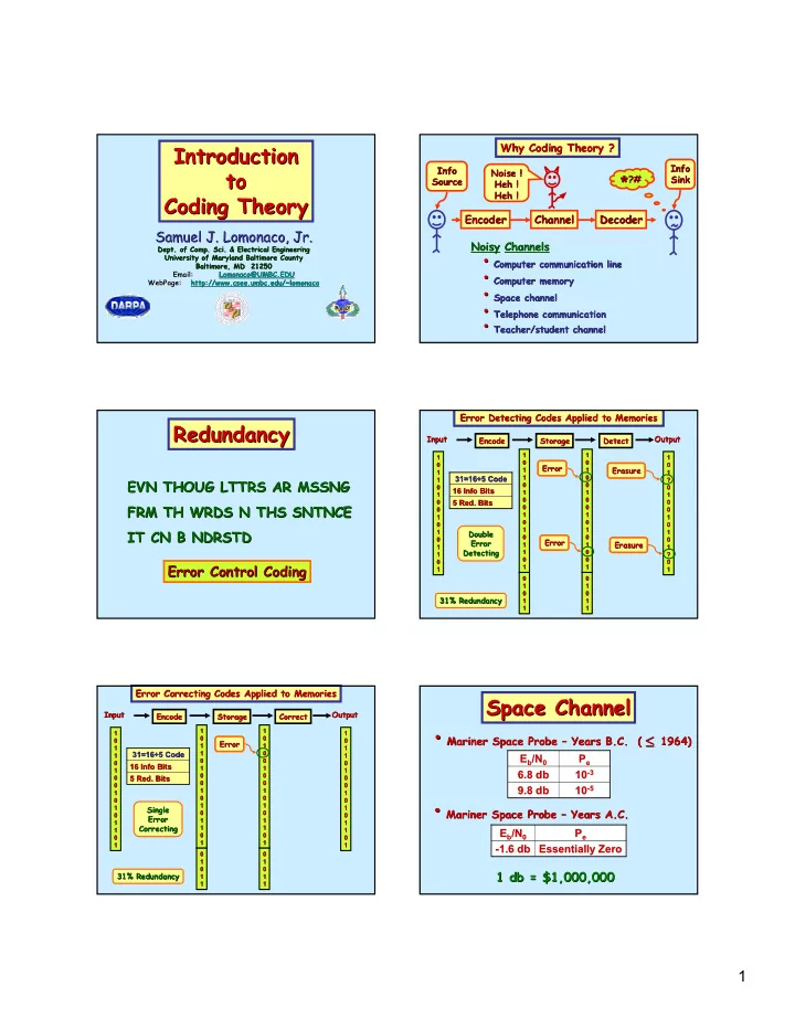
Introduction Introduction to to Coding Theory Coding Theory

Why Coding Theory ? Why Coding Theory ? Channel Channel Encoder Encoder Decoder Decoder

Info Info Source Source Info Info Sink Sink Noise ! Noise ! Heh ! Heh ! Heh ! Heh !

• ?#

?#

Noisy Noisy Channels Channels

• Computer communication line

Computer communication line

• Computer memory

Computer memory

• Space channel

Space channel

• Telephone communication

Telephone communication

• Teacher/student channel

Teacher/student channel

Redundancy Redundancy

EVN THOUG LTTRS AR MSSNG EVN THOUG LTTRS AR MSSNG FRM TH WRDS N THS SNTNCE FRM TH WRDS N THS SNTNCE IT CN B NDRSTD IT CN B NDRSTD Error Control Coding Error Control Coding

Error Detecting Codes Applied to Memories Error Detecting Codes Applied to Memories

Storage Storage Encode Encode Detect Detect Input Input Output Output

1 1 1 1 1 1 1 1 1 1 1 1 1 1 1 1 1 1 1 1 1 1 1 1 1 1 1 1 1 1 1 1 1 1 1 1 1 1 1 1 1 1 1 1 1 1 ? ? 1 1 1 1 1 1 1 1 ? ? 1 1 1 1 1 1 1 1 1 1 1 1 1 1 1 1 1 1 1 1 1 1

Error Error 5 Red. Bits 5 Red. Bits 16 Info Bits 16 Info Bits 31=16+5 Code 31=16+5 Code Double Double Error Error Detecting Detecting 31% Redundancy 31% Redundancy Error Error Erasure Erasure Erasure Erasure

Error Correcting Codes Applied to Memories Error Correcting Codes Applied to Memories

Storage Storage Encode Encode Correct Correct Input Input Output Output

1 1 1 1 1 1 1 1 1 1 1 1 1 1 1 1 1 1 1 1 1 1 1 1 1 1 1 1 1 1 1 1 1 1 1 1 1 1 1 1 1 1 1 1 1 1 1 1 1 1 1 1 1 1 1 1 1 1 1 1 1 1 1 1 1 1 1 1 1 1 1 1 1 1 1 1 1 1 1 1 1 1

Error Error 5 Red. Bits 5 Red. Bits 16 Info Bits 16 Info Bits 31=16+5 Code 31=16+5 Code Single Single Error Error Correcting Correcting 31% Redundancy 31% Redundancy

Space Channel Space Channel

• Mariner Space Probe

Mariner Space Probe – – Years B.C. ( 1964) Years B.C. ( 1964)

≤ ≤

10 10-

• 5

5

9.8 db 9.8 db 10 10-

• 3

3

6.8 db 6.8 db P Pe

e

E Eb

b/N

/N0

• Mariner Space Probe

Mariner Space Probe – – Years A.C. Years A.C. Essentially Zero Essentially Zero

• 1.6 db

1.6 db P Pe

e

E Eb

b/N

/N0

1 db = $1,000,000 1 db = $1,000,000

SLIDE 2

2

Types of Channels Types of Channels

1

p p

1

1 p − 1 p −

1 p − 1 p −

1 1 ?

p p Binary Symmetric Channel (BSC) Binary Symmetric Channel (BSC) Binary Erasure Channel (BEC) Binary Erasure Channel (BEC)

Erasure Erasure

2 2-

• Repeat Code

Repeat Code 11 11 1 1 00 00 Code Words Code Words

• Info. Words
• Info. Words

If we use If we use BEC BEC with with probability of transition probability of transition p = 10 p = 10-

• 2

2,

, then the then the probability probability P PU

U of undetectable error is

• f undetectable error is

2 4

10

U

P p

−

= = = = # 1 # 2 Info Bits Rate R All Bits = = = = =

Moreover, Moreover, Detects all single errors Detects all single errors

A Surprise in Communication Theory A Surprise in Communication Theory

2

10−

4

10−

6

10−

8

10−

10

10−

12

10−

14

10−

1 1

1 11

1 5 1 7 1 9 1 3

• Prob. Of Msg. Error
• Prob. Of Msg. Error

Info Bits Msg Rate All Bits =

C

Channel Channel Capacity Capacity Repetition Repetition Coding Coding Limit Given Limit Given by Shannon by Shannon’ ’s s Theorem Theorem

ε

Choose as Choose as small as small as you like you like

Shannon Shannon’ ’s Theorem s Theorem

Within a large class of coding schemes Within a large class of coding schemes there exist some schemes there exist some schemes – – nearly all, nearly all, actually actually – – that give arbitrarily low error that give arbitrarily low error rates at any information rate up to a rates at any information rate up to a critical rate critical rate C C, called , called channel capacity channel capacity. . Folk Theorem Folk Theorem

“ “All codes are good, except those we can think of. All codes are good, except those we can think of.” ”

Hamming (8,4) 4 Code Hamming (8,4) 4 Code

1111 1111 1111 1111 1111 1111 0010 1110 0010 1110 1110 1110 1000 1101 1000 1101 1101 1101 0101 1100 0101 1100 1100 1100 0100 1011 0100 1011 1011 1011 1001 1010 1001 1010 1010 1010 0011 1001 0011 1001 1001 1001 1110 1000 1110 1000 1000 1000 0001 0111 0001 0111 0111 0111 1100 0110 1100 0110 0110 0110 0110 0101 0110 0101 0101 0101 1011 0100 1011 0100 0100 0100 1010 0011 1010 0011 0011 0011 0111 0010 0111 0010 0010 0010 1101 0001 1101 0001 0001 0001 0000 0000 0000 0000 0000 0000 Code Words Code Words Info Words Info Words

• Corrects all single errors

Corrects all single errors

• Detects all single, double,

Detects all single, double, and triple errors and triple errors We will now apply this code We will now apply this code code code to the BEC with to the BEC with p=10 p=10-

• 2

2

• Rate

Rate R = 1/2 R = 1/2

8 8 8 4 4 4

(1 ) (1 )

k k U k k

P C p p C p p

−

< − < − ≈ −

∑

( ) ( ) ( )

4 4 2 2

70 10 1 10

U

P

− − − −

∴ < ∴ < −

7

6.72 10

U

P

−

∴ < ∴ < ×

• A

A block code block code is a code that uses sequences is a code that uses sequences

• f n channel symbols, or
• f n channel symbols, or n

n-

• tuples

tuples. . Types of Codes Types of Codes Only certain selected Only certain selected n n-

• tuples

tuples, called , called code blocks code blocks or

• r code words

code words are sent. are sent.

• Convolutional

Convolutional Codes: Codes: Each output bit depends on all the previous Each output bit depends on all the previous bits. bits.

SLIDE 3

3

Decoding Table for a Block Code Decoding Table for a Block Code

00001 00001 11111 11111 10100 10100 01010 01010 10101 10101 01011 01011 00000 00000 11110 11110 11101 11101 00011 00011 10110 10110 01000 01000 00101 00101 11011 11011 01110 01110 10000 10000 01001 01001 10111 10111 00010 00010 11100 11100 01111 01111 10001 10001 00100 00100 11010 11010 01100 01100 10010 10010 00111 00111 11001 11001 01101 01101 10011 10011 00110 00110 11000 11000

Received Received Words Words Codewords Codewords

Terminology Terminology

00 01 10 11 11000 00110 10011 01101

Info Info Words Words Code Code Words Words Encoding Encoding Procedure Procedure Code Code

Convolutional Convolutional Codes Codes

1 2 1 0 n n

a a aaa

+

• 1

2 1 0 n n

b b bbb

+

• Convolver

Convolver Infinite Infinite Input Input Infinite Infinite Output Output

Types of Error Correcting Codes Types of Error Correcting Codes

Block Codes Block Codes

• Orthogonal Codes

Orthogonal Codes

• Linear Codes

Linear Codes

• Cyclic Codes

Cyclic Codes

• BCH Codes

BCH Codes

Convolutional Convolutional Codes Codes

• Threshold Decoding

Threshold Decoding

• Sequential Decoding

Sequential Decoding

Block Codes Block Codes

Non Non-

• Linear

Linear Linear Linear Cyclic Cyclic BCH BCH Def.

• Def. A

A code code is a set of binary vectors of is a set of binary vectors of the same fixed length the same fixed length Definitions Definitions Parameters Parameters of codes

• f codes

n = n = length length of code vectors

• f code vectors

R = R = code code rate rate = = (# info bits)/n (# info bits)/n P PU

U =

= Prob.

• Prob. of undetectable error
• f undetectable error

SLIDE 4

4

Problem: Problem: P PU

U depends on the channel

depends on the channel Def.

• Def. Let

Let u u and and v v be n bit vectors. be n bit vectors. The The Hamming Hamming distance distance H(u,v H(u,v) ) between between u u and and v v is the number of bits at which is the number of bits at which they differ. they differ.

( ) ( )

0110,1011 3 H =

( ) ( )

10011, 00011 1 H =

For example, For example, Problem: Problem: P PU

U depends on the channel (Cont.)

depends on the channel (Cont.) Def. Def. The The Hamming Hamming weight weight H(u H(u) ) of

• f u

u is is the number of the number of 1 1’ ’s in s in u u. . For example, For example,

( ) ( )

0110 2 H =

Please also note that Please also note that

( ) ( ) ( )

, H u v H u v = + = +

Def. Def. Let Let V V be a code. Then the be a code. Then the minimum minimum distance distance d(V d(V) ) is is

Problem: Problem: P PU

U depends on the channel (Cont.)

depends on the channel (Cont.)

( ) ( )

( ) , | , u v d V Min H u v u v V ≠   =   ∈  

Observation: Observation:

(1 ) (1 )

n d n d n n n n U d n

P C p p C p p

− − − −

≤ − ≤ − + + −

• So channel independent

So channel independent Code Parameters Code Parameters are: are:

n = n = length length of code vectors

• f code vectors

R = R = code code rate rate = = (# info bits)/n (# info bits)/n d = d = minimum minimum distance distance

A Recurring Theme A Recurring Theme

Add More Algebra Add More Algebra & Gain & Gain

• A trade of space for time, i.e., memory

A trade of space for time, i.e., memory for computation for computation

• Simplifications

Simplifications

Linear Codes Linear Codes

Enter stage right Enter stage right … … Addition Addition We now adjoin We now adjoin addition addition “ “+ +” ” to the to the code space code space

Linear Codes Linear Codes

( ) ( ) { } 2 0,1 , , GF = + = + = i

Galois field Galois field of two

• f two elts

elts. . 1 1 1 1 1 1 1 1 + + 1 1 1 1 1 1

i

( ) ( ) { }

1 2

(2) , , , : (2)

n n n i

E GF b b b b GF i = = = = ∈ ∀ …

( ) ( ) ( ) ( )

1 2 1 2 1 1 2 2

, , , ', ', , ' ', ', , '

n n n n

b b b b b b b b b b b b + = + = + + + … … … ( ) ( ) ( )

1 2 1 2

, , , , , , , (2)

n n

a b b b ab ab ab a G F = ∈ = ∈ … …

= n = n-

• dim

dim vector space over vector space over GF(2) GF(2)

, ,

n

E + i

SLIDE 5

5

Linear Codes Linear Codes

Def. Def. A A linear linear code code V V is a subspace of is a subspace of E E, , i.e., i.e., V V is linear is linear iff iff

, u v V u v V ∈ ⇒ + ∈ + ∈

Parameters Parameters of linear codes:

• f linear codes:

n = n = length length of code vectors

• f code vectors

k = k = dim(V dim(V) = log ) = log2

2(#V) = # Info. Bits

(#V) = # Info. Bits d = d = d(V d(V) = ) = minimum minimum distance distance V V is said to be a linear is said to be a linear ( (n,k n,k) d ) d code code

Length Length Dim Dim

• Min. Dist.
• Min. Dist.

NOTE: NOTE: R= R=k/n k/n

A Simplification A Simplification

• Min. Dist. = Min. Non
• Min. Dist. = Min. Non-
• Zero Wt.

Zero Wt. , ( ) ( , ): u v V d V Min H u v u v ∈   =   ≠   ( ): u V Min H u u ∈   =   ≠  

Error Model Error Model

v

Sent Sent Vector Vector

r v ε = + = +

Received Received Vector Vector

ε

Error Error Vector Vector

An example of the Error Model An example of the Error Model

001110 v =

Sent Sent Vector Vector

r v ε = + = +

Received Received Vector Vector

000010 ε =

Error Error Vector Vector

001100 =

001100 r = 001110 v = 000010 ε =

+

An Example: The Hamming (7,4) 3 Code An Example: The Hamming (7,4) 3 Code

111 1111 111 1111 1111 1111 010 1110 010 1110 1110 1110 000 1101 000 1101 1101 1101 101 1100 101 1100 1100 1100 100 1011 100 1011 1011 1011 001 1010 001 1010 1010 1010 011 1001 011 1001 1001 1001 110 1000 110 1000 1000 1000 Codeword Codeword Infoword Infoword 001 0111 001 0111 0111 0111 100 0110 100 0110 0110 0110 110 0101 110 0101 0101 0101 011 0100 011 0100 0100 0100 010 0011 010 0011 0011 0011 111 0010 111 0010 0010 0010 101 0001 101 0001 0001 0001 000 0000 000 0000 0000 0000 Codeword Codeword Infoword Infoword

( ) ( ) ( )

3 2 1 6 5 4 3 2 1

, , , , , , , , , b b b b b b b b b b b

• 6

2 3

b b b b = + = + +

5 1 2

b b b b = + = + +

4 1 2 3

b b b b = + = + +

where where

Infoword Infoword Codeword Codeword

• A

A Linear Linear Code Code The Hamming (7,4) 3 Code (Cont.) The Hamming (7,4) 3 Code (Cont.)

( ) ( ) ( )

3 2 1 6 5 4 3 2 1

1 0 1 1 0 0 0 1 1 1 0 1 0 0 , , , , , , , , , 0 1 1 0 0 1 0 1 1 1 0 0 0 1 b b b b b b b b b b b      =      

Generator Generator Matrix Matrix G G

Infoword Infoword Codeword Codeword

{ }

7 4

: . . V v E u E s t uG v = ∈ = ∈ ∃ ∈ =

The rows of The rows of G G span the linear code span the linear code V V. .

SLIDE 6

6

The Hamming (7,4) 3 Code (Cont.) The Hamming (7,4) 3 Code (Cont.)

( ) ( ) ( ) ( )

6 5 4 3 2 1

1 0 0 1 1 0 1 , , , , , , 0 1 0 0 1 1 1 0,0,0 0 0 1 1 1 1 0

T

b b b b b b b     =      

Codeword Codeword

Parity Parity Check Check Matrix Matrix H HT

T

{ }

7 : T

V v E vH = ∈ = ∈ =

• The rows of

The rows of H HT

T span the linear code

span the linear code . .

V ⊥

Linear Codes Linear Codes

• The rows of the

The rows of the generator matrix generator matrix G G span span the code the code V V. .

• The columns of the

The columns of the parity check matrix parity check matrix H H span the span the dual code dual code . .

V ⊥

Linear Codes Linear Codes

Def. Def. Let Let V V be a linear code in be a linear code in E En

• n. Then

. Then the the dual dual code code V V⊥

⊥ of

• f V

V is is where where

{ }

: 0,

n

V v E v u u V

⊥ =

∈ = ∈ = ∀ ∈ i

i i i

v u v u = ∑ i

Linear Codes Linear Codes

Observation: Observation:

T

v V vH ∈ ⇔ ∈ ⇔ =

( ) ( )

T T T T

v e H vH eH eH + = + = + =

Hence, Hence, Def.

• Def. Let be a received vector. Then

Let be a received vector. Then is called the is called the syndrome syndrome of .

• f .

r

• r
• T

r H

• i

The syndrome depends only on the error The syndrome depends only on the error pattern pattern e e. . Maximum Likelihood Decoding Maximum Likelihood Decoding

110001 110001 111111 111111 100100 100100 010010 010010 101010 101010 011100 011100 000111 000111 001001 001001 011000 011000 010110 010110 001101 001101 111011 111011 000011 000011 110101 110101 101110 101110 100000 100000 101000 101000 100110 100110 111101 111101 001011 001011 110011 110011 000101 000101 011110 011110 010000 010000 110000 110000 111110 111110 100101 100101 010011 010011 101011 101011 011101 011101 000110 000110 001000 001000 111100 111100 110010 110010 101001 101001 011111 011111 100111 100111 010001 010001 001010 001010 000100 000100 111010 111010 110100 110100 101111 101111 011001 011001 100001 100001 010111 010111 001100 001100 000010 000010 111001 111001 110111 110111 101100 101100 011010 011010 100010 100010 010100 010100 001111 001111 000001 000001 11100 11100 110110 110110 101101 101101 011011 011011 100011 100011 010101 010101 001110 001110 000000 000000

Code Code Coset Coset Leaders Leaders Error Patterns Error Patterns

Standard Standard Array Array for a Linear for a Linear (6,3) 3 (6,3) 3 Code Code

Decoding Decoding Table Table

Maximum Likelihood Decoding Maximum Likelihood Decoding

Syndrome Syndrome Error Error 111 111 001001 001001 011 011 100000 100000 101 101 010000 010000 110 110 001000 001000 100 100 000100 000100 010 010 000010 000010 001 001 000001 000001 000 000 000000 000000

Most Probable Error Most Probable Error Pattern for Given Syndrome Pattern for Given Syndrome Error/Syndrome Error/Syndrome Table Table

SLIDE 7

7

A Recurring Theme A Recurring Theme

Add More Algebra Add More Algebra & Gain & Gain

• A trade of space for time, i.e., memory

A trade of space for time, i.e., memory for computation for computation

• Simplifications

Simplifications

Cyclic Codes Cyclic Codes

Enter stage right Enter stage right … … Multiplication Multiplication We now adjoin We now adjoin Multiplication Multiplication “ “•

• ”

” to the code space to the code space

Cyclic Codes: Preliminaries Cyclic Codes: Preliminaries

Each Each n n-

• bit binary number

bit binary number can be considered to can be considered to be a polynomial be a polynomial with coefficients over with coefficients over GF(2) GF(2) . .

1 2 3 4 5 6 7

10101011 1 1 1 1 1 x x x x x x x x = + + + + + + + + + + + i i i i i i i i

2 4 6 7

1 x x x x = + + + + + + + +

Cyclic Codes: Preliminaries Cyclic Codes: Preliminaries

1 1 1 1 1 1 1 1 +

2 3 3 2

1 1 x x x x x x + + + + + + + + + + + + + +

Addition Addition

Cyclic Codes: Preliminaries Cyclic Codes: Preliminaries 1 1 1 1 1 1 1 1 1 1 1 1 ×

2 2 3 2 4 2 3 4

1 x x x x x x x x x x x + × + × + + + + + + + + +

Multiplication Multiplication

Cyclic Codes: Preliminaries Cyclic Codes: Preliminaries

Problem Problem: : Multiplication of code vectors Multiplication of code vectors (thought of as polynomials) may increase (thought of as polynomials) may increase code vector length. code vector length. Example Example: :

( ) ( ) ( )

( ) ( ) ( )

2 2

101 011 1 x x x = + = + + i i

2 3 4

01111 x x x x = + + + + + + =

Both Both Length Length 3 3 Length Length 5 5

SLIDE 8

8

Cyclic Codes: Preliminaries Cyclic Codes: Preliminaries

A quick way to fix the problem: A quick way to fix the problem: Assume Assume x xn

n=1

=1 or

• r x

xn

n+1=0

+1=0, where , where n n denotes the codeword length. denotes the codeword length. Example: Example: n=3 n=3 Therefore, Therefore, x x3

3=1

=1

4

, x x ∴ = ∴ =

5 2,

x x ∴ = ∴ =

6 3

1 x x ∴ = ∴ = =

2 3 4 2

01111 1 x x x x x x x ∴ = + + + + + = + + + + + ( ) ( )

2 2

1 1 1 1 x x x x x = + = + + + = + = + + +

2

1 101 x = + = + =

Cyclic Codes: Preliminaries Cyclic Codes: Preliminaries

Hence, under this identification, the Hence, under this identification, the linear space linear space

( ) ( ) { }

1 1

, , , , : (2) ,

n n i

E b b b b GF

−

+ = + = ∈ + …

becomes a becomes a RING

RING

( ) ( ) { } { }

1 1 1

(2)[ ], , : (2) , , 1

n n n i n

G F x R b bx b x b G F x

− −

= + = + = + + + ∈ + + i

• i

Cyclic Codes Cyclic Codes Def. Def. A linear code A linear code V V in in E En

n is a

is a cyclic code cyclic code if if

( ) ( ) ( )

1 1 1 1 2

, , , , , , ,

n n n

v v v V v v v v V

− − − − −

∈ ⇒ ∈

• Identify

Identify with the polynomial with the polynomial

( ) ( )

1 1

, , ,

n

v v v −

• 2

1 1 2 1

( )

n n

v x v v x v x v x −

−

= + = + + + +

• Then

Then a cyclic shift is a cyclic shift is

( ) ( ) v x x v x

• i

in the ring in the ring

( ) ( )

(2)[ ]/ 1

n n

E GF x x = + = +

Cyclic Codes Cyclic Codes

Proposition. Proposition. A cyclic code V is an A cyclic code V is an ideal ideal in in the ring , i.e., the ring , i.e.,

1) 1) 2) 2)

( ) ( )

(2)[ ]/ 1

n

GF x x +

, ' ' v v V v v V ∈ ⇒ − ∈ − ∈

,

n

u E v V u v V ∈ ∈ ∈ ∈ ⇒ ∈ i

Generator Polynomial of a Cyclic Code Generator Polynomial of a Cyclic Code

But But E En

n

is a principal ideal domain. is a principal ideal domain. Hence, for every cyclic code Hence, for every cyclic code V V, there , there exists a polynomial exists a polynomial g(x g(x) ) such that such that

( ) ( ) {

}

( ) ( ) ( ): ( )

n

V g x u x v x u x E = = = = ∈

We choose We choose g(x g(x) ) so that it is a factor of so that it is a factor of 1+x 1+xn

n . Such a choice is

. Such a choice is unique unique. . The polynomial The polynomial g(x g(x) ) is called a is called a generator generator polynomial polynomial of the cyclic code

• f the cyclic code V

V . . Proposition. Proposition. k = k = dim(V dim(V) = n ) = n -

• deg(g

deg(g) )

Generator Polynomial of a Cyclic Code Generator Polynomial of a Cyclic Code

Proposition. Proposition. The generator matrix The generator matrix G G

• f
• f

a cyclic code can be written in the form a cyclic code can be written in the form

1

( ) ( ) ( )

k

g x xg x G x g x

−

      =      

SLIDE 9

9

Encoding and Decoding Procedures for Cyclic Codes Encoding and Decoding Procedures for Cyclic Codes

Encoding Procedure = Multiplication Encoding Procedure = Multiplication g(x g(x) ) Decoding Procedure = Division by Decoding Procedure = Division by g(x g(x) )

( ) ( ) ( ) i x i x g x

• ( )

( )/ ( ) r x r x g x

• An Example

An Example

Consider the cyclic code Consider the cyclic code V V given by the generator given by the generator polynomial polynomial g(x g(x) = 1+x+x ) = 1+x+x3

3

Let Let n n be the smallest positive integer be the smallest positive integer s.t s.t. . g(x g(x) (1+x ) (1+xn

n)

) Then Then n = 7 n = 7 and and dim(V dim(V) = k = n ) = k = n – – deg(g deg(g) = 7 ) = 7 – – 3 = 4 3 = 4

This is the This is the Hamming Hamming (7,4) 3 (7,4) 3 code. code.

If If i(x i(x) = 1+x ) = 1+x, then the encoded vector is , then the encoded vector is

( ) ( )(

) ( )

3 3 2 4

1 1 1 x x x x x x x x + + + = + + + + + + + + +

2 3 4

1 x x x = + + + + + + 1100 1011100 ∴

• Another Recurring Theme

Another Recurring Theme

Algebra = Computing Algebra = Computing

Encoding Circuit = Encoding Circuit = Circuit Circuit which Multiplies by which Multiplies by g(x g(x) )

1100 1011100

Infoword Infoword Codeword Codeword

1 1 1 1 1 1 1 1 1 1 1 1 1 1 1 1 1 1 1 1 1 1 1 1 1 1 1 1 1 1 1 1 1 1 1 1 1 1 1 1 1 1 1 1 1 1 1 1 1 1 1 1

A circuit which multiplies by A circuit which multiplies by 1+x+x 1+x+x3

3 Input Input State State Output Output 1 1 x x3

3

x x2

2

x x

General Encoding Circuit which Multiplies General Encoding Circuit which Multiplies by an Arbitrary Generator Polynomial by an Arbitrary Generator Polynomial g(x g(x) )

… …

g g0 g gn

n

g gn

n-

• 1

1

g g2

2

g g1

1

…

Linear Circuit for multiplying by Linear Circuit for multiplying by g(x)=g0+g1x+g2x2+ … +gn-1xn-1+gnxn

Input Input

( ) i x

( ) ( ) i x g x

Output Output

1 1 1 1 1 1 1 1 1 1 1 1 1 1 1 1 1 1 1 1 1 1 1 1 1 1 1 1 1 1 1 1

Decoding Circuit = Decoding Circuit = Circuit Circuit that Divides by that Divides by g(x g(x) = 1+x+x ) = 1+x+x3

3

3 ( )

x g x =

Input Input State State

2

( ) Sx x x = = = = +

Initial State Initial State Syndrome Syndrome Input Input

SLIDE 10

10

General Encoding Circuit which Divides by General Encoding Circuit which Divides by an Arbitrary Generator Polynomial an Arbitrary Generator Polynomial g(x g(x) )

…

Linear Circuit for dividing by Linear Circuit for dividing by g(x)=g0+g1x+g2x2+ … +gn-1xn-1+gnxn

Output Output

( )/ ( ) i x g x

Input Input

( ) i x

… …

• g

g0 g gn

n

• 1

1

• g

gn

n-

• 1

1

• g

g2

2

• g

g1

1

An Example An Example

Output Output

( ) ( )

3

( )/ 1 i x x x + + + +

( ) i x

Input Input

Linear Circuit for dividing by Linear Circuit for dividing by g(x)=1+x+x3

A Recurring Theme A Recurring Theme

Add More Algebra Add More Algebra & Gain & Gain

• A trade of space for time, i.e., memory

A trade of space for time, i.e., memory for computation for computation

• Simplifications

Simplifications

BCH Codes BCH Codes

Enter stage right Enter stage right … … More Algebraic Structure More Algebraic Structure

BCH = Bose BCH = Bose-

• Chaudhuri

Chaudhuri-

• Hocquenghem

Hocquenghem

Galois Fields (Characteristic 2) Galois Fields (Characteristic 2)

GF(2 GF(2k

k) = GF[2]/(p(x))

) = GF[2]/(p(x)) , where , where 1) 1) deg( deg( p(x p(x) ) = k ) ) = k 2) 2) p(x p(x) ) is is irreducible irreducible 3) 3) p(x p(x) ) is is primitive primitive, i.e., the residue , i.e., the residue class class ξ ξ containing containing x x generates the generates the multiplicative group of multiplicative group of GF(2 GF(2k

k).

).

Galois Fields (Characteristic 2) Galois Fields (Characteristic 2)

Simplified Simplified Approach Approach GF(2 GF(2k

k) =

) = polynomials in polynomials in ξ ξ subject to the subject to the relation relation p( p(ξ ξ) = 0 ) = 0 . . Example Example: : Construction of Construction of GF(2 GF(23

3)

) Let Let p(x p(x) = ) = 1+ 1+ξ+ξ 1+ 1+ξ+ξ3

3 ; hence

; hence ξ ξ3

3 = 1

= 1+ξ = 1 = 1+ξ . . Therefore, every polynomial in Therefore, every polynomial in ξ ξ reduces reduces to one of the form to one of the form a a0

0+a

+a1

1x+a

x+a2

2x

x2

2 ,

, where where a ai

i e

e GF(2) GF(2) for for i = 0,1,2 i = 0,1,2

SLIDE 11

11

Example (Cont.) Example (Cont.)

110 110 110 110 = = 1+ 1+ξ 1+ 1+ξ = = ξ ξ4

4

011 011 011 011 = = ξ ξ + +ξ ξ ξ + +ξ2

2

= = ξ ξ5

5

111 111 111 111 = = 1+ 1+ξ+ξ 1+ 1+ξ+ξ2

2

= = ξ ξ6

6

101 101 101 101 = = 1 1 +ξ 1 1 +ξ2

2

= = ξ ξ7

7

001 001 001 001 = = ξ ξ2

2

= = ξ ξ2

2

010 010 010 010 = = ξ ξ = = ξ ξ1

1

100 100 100 100 = = 1 1 = = ξ ξ0 000 000 000 000 = = = = where where a a0

0 + a

+ a1

1ξ

ξ ξ ξ + a + a2

2ξ

ξ2

2

a a0

0 a

a1

1 a

a2

2

GF(2 GF(23

3)

)

Example (Cont.) Example (Cont.)

We can create other Galois fields using We can create other Galois fields using the following the following “ “relations relations” ” GF(2 GF(22

2)

) with the relation with the relation 1+ 1+ξ+ξ 1+ 1+ξ+ξ2

2 = 0

= 0 = 0 = 0 GF(2 GF(23

3)

) “ “ “ “ “ “ 1+ 1+ξ+ξ 1+ 1+ξ+ξ3

3 = 0

= 0 = 0 = 0 GF(2 GF(24

4)

) “ “ “ “ “ “ 1+ 1+ξ+ξ 1+ 1+ξ+ξ4

4 = 0

= 0 = 0 = 0 GF(2 GF(25

5)

) “ “ “ “ “ “ 1+ 1+ξ 1+ 1+ξ2

2+ξ

+ξ +ξ +ξ5

5 = 0

= 0 = 0 = 0 GF(2 GF(26

6)

) “ “ “ “ “ “ 1+ 1+ξ+ξ 1+ 1+ξ+ξ6

6 = 0

= 0 = 0 = 0

Another way to describe cyclic linear codes Another way to describe cyclic linear codes

Another way to describe a cyclic code, i.e., in terms Another way to describe a cyclic code, i.e., in terms

• f the roots of the generator polynomial
• f the roots of the generator polynomial g(x

g(x) ) . . V = ( V = ( g(x g(x) ) = { ) ) = { h(x h(x) : ) : h( h(α α) = 0 ) = 0 for all roots of for all roots of g(x g(x) } ) }

Example.

• Example. Let

Let V = V = Hamming ( Hamming (7,4) 3 7,4) 3 linear code. linear code. Then Then g(x g(x) = 1+x+x ) = 1+x+x3

3, and the roots of

, and the roots of g(x g(x) ) are are ξ ξ, , ξ ξ2

2,

, ξ ξ4

4 in GF(2

in GF(23

3). Hence, the linear code is

). Hence, the linear code is V ={ V ={ h(x h(x) : ) : h( h(ξ ξ) = h( ) = h(ξ ξ2

2) = h(

) = h(ξ ξ4

4) =0 }

) =0 } Moreover, the Moreover, the syndrome syndrome is given by is given by r( r(ξ ξ) = ) = h( h(ξ ξ)+e( )+e(ξ ξ) = ) = e( e(ξ ξ) )

BCH Codes BCH Codes

Def Def. . Let Let ξ ξ be a primitive root of be a primitive root of GF(2 GF(2m

m)

). A . A cyclic linear code cyclic linear code V V generated by a polynomial generated by a polynomial g(x g(x) ) is a is a BCH BCH code code with with design design parameter parameter δ δ if if g(x g(x) ) is the polynomial of smallest degree over is the polynomial of smallest degree over GF(2) GF(2) having having

ξ ξ, , ξ ξ2

2,

,ξ ξ3

3,

, … … , , ξ ξδ

δ-

• 1

1

as roots. as roots.

BCH Codes (Cont.) BCH Codes (Cont.)

Id Id δ δ = 2t = 2t0

0+1

+1. Then the BCH code can . Then the BCH code can correct t0 errors, and detect 2t0 errors. correct t0 errors, and detect 2t0 errors. Such a BCH code is a cyclic linear Such a BCH code is a cyclic linear (2 (2m

m-

• 1,k) d

1,k) d code, where code, where

2 1

m

k mt ≥ − ≥ − − d δ ≥

An Example An Example

Let Let ξ ξ be a primitive root of be a primitive root of GF(24) GF(24) , where , where p(x p(x) = 1+x ) = 1+x3

3+x

+x4

4

Let Let V V be the cyclic linear code consisting of all be the cyclic linear code consisting of all vectors vectors h(x h(x) ) having the roots having the roots

ξ, ξ, ξ ξ ξ, ξ, ξ ξ2

2, ξ

, ξ , ξ , ξ3

3, ξ

, ξ , ξ , ξ4

4, ξ

, ξ , ξ , ξ5

5, ξ

, ξ , ξ , ξ7

7− −1 1

Then Then ξ , ξ

ξ , ξ ξ , ξ ξ , ξ2

2, ξ

, ξ , ξ , ξ4

4 4 4 , ξ

, ξ , ξ , ξ8

8

ξ ξ3

3, ξ

, ξ , ξ , ξ6

6, ξ

, ξ , ξ , ξ12

12 12 12, ξ

, ξ , ξ , ξ9

9

ξ ξ5

5, ξ

, ξ , ξ , ξ10

10 10 10

m m1

1(x)=m

(x)=m2

2(x)=m

(x)=m4

4(x) (deg 4)

(x) (deg 4) m m3

3(x)=m

(x)=m6

6(x) (deg 4)

(x) (deg 4) m m5

5(x) (deg 2)

(x) (deg 2) So So g(x g(x) = m ) = m1

1(x)m

(x)m3

3(x)m

(x)m5

5(x)

(x) ; and hence of ; and hence of deg 10 deg 10 Therefore, Therefore, (2 (2m

m-

• 1

1,k) d = (15,5) d

,k) d = (15,5) d, where , where d 7 d 7

≥

SLIDE 12

12

The End The End