
SLIDE 1
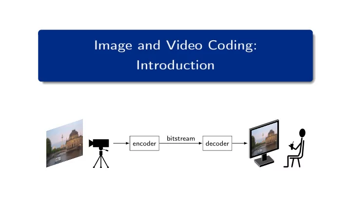
Image and Video Coding: Introduction bitstream encoder decoder - - PowerPoint PPT Presentation
Image and Video Coding: Introduction bitstream encoder decoder Motivation Image and Video Coding video bitstream bitstream video transmission encoder decoder or storage data data Main Goal of Image and Video Coding Efficient
Motivation
bitstream bitstream video data video data
Heiko Schwarz (Freie Universität Berlin) — Image and Video Coding: Introduction 2 / 48
Motivation
Heiko Schwarz (Freie Universität Berlin) — Image and Video Coding: Introduction 3 / 48
Motivation
[ Cisco: “The Zettabyte Era: Trends and Analysis”, 2017 ]
Heiko Schwarz (Freie Universität Berlin) — Image and Video Coding: Introduction 4 / 48
Source Data for Image and Video Coding / Gray-Level Images
x y H W
Heiko Schwarz (Freie Universität Berlin) — Image and Video Coding: Introduction 5 / 48
Source Data for Image and Video Coding / Gray-Level Images
Heiko Schwarz (Freie Universität Berlin) — Image and Video Coding: Introduction 6 / 48
Source Data for Image and Video Coding / Gray-Level Images
— Image and Video Coding: Introduction 6 / 48
Source Data for Image and Video Coding / Gray-Level Images
Heiko Schwarz (Freie Universität Berlin) — Image and Video Coding: Introduction 7 / 48
Source Data for Image and Video Coding / Color Images
Heiko Schwarz (Freie Universität Berlin) — Image and Video Coding: Introduction 8 / 48
Source Data for Image and Video Coding / Color Images
3×3
Heiko Schwarz (Freie Universität Berlin) — Image and Video Coding: Introduction 9 / 48
Source Data for Image and Video Coding / Color Images
Heiko Schwarz (Freie Universität Berlin) — Image and Video Coding: Introduction 10 / 48
Source Data for Image and Video Coding / Color Images
— Image and Video Coding: Introduction 11 / 48
Source Data for Image and Video Coding / Videos
Heiko Schwarz (Freie Universität Berlin) — Image and Video Coding: Introduction 12 / 48
Source Data for Image and Video Coding / Videos
Heiko Schwarz (Freie Universität Berlin) — Image and Video Coding: Introduction 13 / 48
Source Data for Image and Video Coding / Raw Data Rate
Heiko Schwarz (Freie Universität Berlin) — Image and Video Coding: Introduction 14 / 48
The Image and Video Coding Problem / Video Communication
capture raw input data samples raw input data samples pre- processing video encoder video encoder transmission channel (can be replaced by storage) channel encoder modulator channel demodulator channel decoder video decoder video decoder post- processing raw output data samples raw output data samples
perception encoded bitstream received bitstream no transmission errors bitstream
Heiko Schwarz (Freie Universität Berlin) — Image and Video Coding: Introduction 15 / 48
The Image and Video Coding Problem / Video Communication
Heiko Schwarz (Freie Universität Berlin) — Image and Video Coding: Introduction 16 / 48
The Image and Video Coding Problem / Video Communication
Heiko Schwarz (Freie Universität Berlin) — Image and Video Coding: Introduction 17 / 48
The Image and Video Coding Problem / The Coding Problem
Heiko Schwarz (Freie Universität Berlin) — Image and Video Coding: Introduction 18 / 48
The Image and Video Coding Problem / The Coding Problem
Heiko Schwarz (Freie Universität Berlin) — Image and Video Coding: Introduction 19 / 48
The Image and Video Coding Problem / Summary
Heiko Schwarz (Freie Universität Berlin) — Image and Video Coding: Introduction 20 / 48
Image Compression Example: JPEG / Overview
2d block transform scalar quantization entropy coding block of samples sequence
2d inverse transform scaling entropy decoding reconstructed block sequence
Heiko Schwarz (Freie Universität Berlin) — Image and Video Coding: Introduction 21 / 48
Image Compression Example: JPEG / Overview
input component input component
partitioned into blocks
partitioned into blocks
97 205 180 129 82 189 160 117 49 184 150 88 64
samples
2d block transform scalar quantization entropy coding
bitstream
2d block transform
1 Partitioning into Blocks 2 Transform Coding of Blocks
a 2D Transform:
Energy compaction
b Quantization:
Approximate signal (remove invisible details)
c Entropy Coding: Represent data with
as little bits as possible
Heiko Schwarz (Freie Universität Berlin) — Image and Video Coding: Introduction 22 / 48
Image Compression Example: JPEG / Transform
Heiko Schwarz (Freie Universität Berlin) — Image and Video Coding: Introduction 23 / 48
Image Compression Example: JPEG / Transform
Heiko Schwarz (Freie Universität Berlin) — Image and Video Coding: Introduction 24 / 48
Image Compression Example: JPEG / Transform
s0 s1 t0 t1
Heiko Schwarz (Freie Universität Berlin) — Image and Video Coding: Introduction 25 / 48
Image Compression Example: JPEG / Transform
block horizontal DCT vertical DCT after 2d DCT
Heiko Schwarz (Freie Universität Berlin) — Image and Video Coding: Introduction 26 / 48
Image Compression Example: JPEG / Transform
input component
partitioned into blocks
97 205 180 129 82 189 160 117 49 184 150 88 64
samples
entropy coding
bitstream
2d block transform 2d block transform
1810 620 159 13 223 −7 −31 8 32 −10 34 −27 −3 18 −34 28 transform coefficients
scalar quantization scalar quantization
Heiko Schwarz (Freie Universität Berlin) — Image and Video Coding: Introduction 27 / 48
Image Compression Example: JPEG / Quantization
Heiko Schwarz (Freie Universität Berlin) — Image and Video Coding: Introduction 28 / 48
Image Compression Example: JPEG / Quantization
input component
partitioned into blocks
97 205 180 129 82 189 160 117 49 184 150 88 64
samples
2d block transform
1810 620 159 13 223 −7 −31 8 32 −10 34 −27 −3 18 −34 28 transform coefficients bitstream
∆ = 100 scalar quantization scalar quantization
18 6 2 2 quantization indexes
entropy coding entropy coding
Heiko Schwarz (Freie Universität Berlin) — Image and Video Coding: Introduction 29 / 48
Image Compression Example: JPEG / Entropy Coding
1 −1 2 −2 3 −3 4 −4 k p(k)
indexes k: 18, 6, 2, 0, 2, 0, · · ·, 0 (16 values) simple: 7 + 7 + 2 · 7 + 12 · 6 = 100 bits better: 10 + 6 + 2 · 4 + 12 · 1 = 36 bits
simple better k codewords codewords 000000 ±1 000001 s 10 0 s ±2 000010 s 10 1 s ±3 000011 s 110 00 s ±4 000100 s 110 01 s ±5 000101 s 110 10 s ±6 000110 s 110 11 s ±7 000111 s 1110 000 s ±8 001000 s 1110 001 s · · · · · · · · · ±14 001110 s 1110 111 s ±15 001111 s 11110 0000 s ±16 010000 s 11110 0001 s ±17 010001 s 11110 0010 s ±18 010010 s 11110 0011 s · · · · · · · · · ±63 111111 s 1111110 000000 s
Heiko Schwarz (Freie Universität Berlin) — Image and Video Coding: Introduction 30 / 48
Image Compression Example: JPEG / Entropy Coding
18 6 2 2 18 6 2 2
scanned k: 18, 6, 2, 0, 0, 2, 0, · · ·, 0 (16 values) new code: 11 + 7 + 5 + 2 · 1 + 5 + 2 = 32 bits
k code with eob (eob) 10 ±1 110 0 s ±2 110 1 s ±3 1110 00 s ±4 1110 01 s ±5 1110 10 s ±6 1110 11 s ±7 11110 000 s ±8 11110 001 s · · · · · · ±14 11110 111 s ±15 111110 0000 s ±16 111110 0001 s ±17 111110 0010 s ±18 111110 0011 s · · · · · · ±63 11111110 000000 s
Heiko Schwarz (Freie Universität Berlin) — Image and Video Coding: Introduction 31 / 48
Image Compression Example: JPEG / Entropy Coding
input component
partitioned into blocks
samples
2d block transform
transform coefficients bitstream
scalar quantization
quantization indexes
∆ = 100
222 199 148 97 205 180 129 82 189 160 117 49 184 150 88 64 1810 620 159 13 223 −7 −31 8 32 −10 34 −27 −3 18 −34 28
entropy coding
18 6 2 2
entropy coding
1111 1000 1101 1101 1011 0100 0110 1010
18 6 2 2
1111 1000 1101 1101 1011 0100 0110 1010
Heiko Schwarz (Freie Universität Berlin) — Image and Video Coding: Introduction 32 / 48
Image Compression Example: JPEG / Decoding
input component
partitioned into blocks
samples
2d block transform
transform coefficients
scalar quantization
quantization indexes
∆ = 100 entropy coding
1111 1000 1101 1101 1011 0100 0110 1010
bitstream bitstream bitstream
entropy decoding
18 6 2 2
entropy decoding
quantization indexes
same indexes
scaling
1800 600 200 200
scaling
reconstructed transform coefficients
∆ = 100
approximation lossy part
2d inverse transform
214 195 142 92 202 184 131 81 185 166 113 63 173 155 102 52
2d inverse transform
reconstructed samples
reconstructed component
approximation
8 4 6 5 3 −4 −2 1 4 −6 4 −14 11 −5 −14 12
difference signal / reconstruction error vs. number of bits trade-off is determined by quantization step size ∆
Heiko Schwarz (Freie Universität Berlin) — Image and Video Coding: Introduction 33 / 48
Image Compression Example: JPEG / JPEG Examples
Heiko Schwarz (Freie Universität Berlin) — Image and Video Coding: Introduction 34 / 48
Image Compression Example: JPEG / JPEG Examples
Heiko Schwarz (Freie Universität Berlin) — Image and Video Coding: Introduction 34 / 48
Image Compression Example: JPEG / JPEG Examples
Heiko Schwarz (Freie Universität Berlin) — Image and Video Coding: Introduction 34 / 48
Image Compression Example: JPEG / JPEG Examples
Heiko Schwarz (Freie Universität Berlin) — Image and Video Coding: Introduction 34 / 48
Image Compression Example: JPEG / JPEG Examples
Heiko Schwarz (Freie Universität Berlin) — Image and Video Coding: Introduction 34 / 48
Image Compression Example: JPEG / JPEG Examples
Heiko Schwarz (Freie Universität Berlin) — Image and Video Coding: Introduction 34 / 48
Image Compression Example: JPEG / Summary
1 Orthogonal Block Transform
2 Scalar Quantization of Transform Coefficients
3 Entropy Coding of Quantization Indexes
Heiko Schwarz (Freie Universität Berlin) — Image and Video Coding: Introduction 35 / 48
Video Coding Basics / Inter-Picture Similarities
Heiko Schwarz (Freie Universität Berlin) — Image and Video Coding: Introduction 36 / 48
Video Coding Basics / Inter-Picture Similarities
Heiko Schwarz (Freie Universität Berlin) — Image and Video Coding: Introduction 37 / 48
Video Coding Basics / Motion-Compensated Prediction
n−1
current original picture sn prediction error un (difference)
1 Get prediction error:
n−1[x, y]
2 Transform coding:
n[x, y]
3 Transmit in bitstream: Quantization indexes {k} 4 Reconstruction:
n[x, y] = s′ n−1[x, y] + u′ n[x, y]
Heiko Schwarz (Freie Universität Berlin) — Image and Video Coding: Introduction 38 / 48
Video Coding Basics / Motion-Compensated Prediction
n−1
current original picture sn prediction error un (MCP)
n−1
1 Get prediction error:
n−1[x + mx, y + my]
2 Transform coding:
n[x, y]
3 Transmit in bitstream: Motion vector (mx, my) and quantization indexes {k} 4 Reconstruction:
n[x, y] = s′ n−1[x + mx, y + my] + u′ n[x, y]
Heiko Schwarz (Freie Universität Berlin) — Image and Video Coding: Introduction 39 / 48
Video Coding Basics / Motion-Compensated Prediction
Heiko Schwarz (Freie Universität Berlin) — Image and Video Coding: Introduction 40 / 48
Video Coding Basics / Video Coding Examples
Heiko Schwarz (Freie Universität Berlin) — Image and Video Coding: Introduction 41 / 48
Coding Efficiency / Measuring Bit Rate and Quality
Heiko Schwarz (Freie Universität Berlin) — Image and Video Coding: Introduction 42 / 48
Coding Efficiency / Measuring Bit Rate and Quality
max
max
N−1
— Image and Video Coding: Introduction 43 / 48
Coding Efficiency / Rate-PSNR Plots
Heiko Schwarz (Freie Universität Berlin) — Image and Video Coding: Introduction 44 / 48
Coding Efficiency / Example: Comparison of JPEG and HEVC
Heiko Schwarz (Freie Universität Berlin) — Image and Video Coding: Introduction 45 / 48
Coding Efficiency / Example: Comparison of JPEG and HEVC
Heiko Schwarz (Freie Universität Berlin) — Image and Video Coding: Introduction 46 / 48
Summary
Heiko Schwarz (Freie Universität Berlin) — Image and Video Coding: Introduction 47 / 48
Summary
Heiko Schwarz (Freie Universität Berlin) — Image and Video Coding: Introduction 48 / 48