
SLIDE 1
Idealized Power Curve
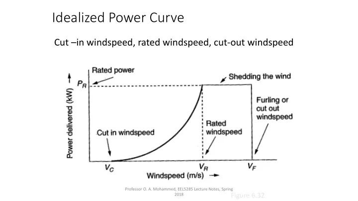
Cut –in windspeed, rated windspeed, cut-out windspeed
Figure 6.32
Professor O. A. Mohammed, EEL5285 Lecture Notes, Spring 2018
Idealized Power Curve Cut in windspeed, rated windspeed, cut-out - - PowerPoint PPT Presentation
Idealized Power Curve Cut in windspeed, rated windspeed, cut-out windspeed Professor O. A. Mohammed, EEL5285 Lecture Notes, Spring Figure 6.32 2018 Idealized Power Curve Before the cut-in windspeed , no net power is generated Then,
Figure 6.32
Professor O. A. Mohammed, EEL5285 Lecture Notes, Spring 2018
Professor O. A. Mohammed, EEL5285 Lecture Notes, Spring 2018
Professor O. A. Mohammed, EEL5285 Lecture Notes, Spring 2018
3 3
avg avg avg
Professor O. A. Mohammed, EEL5285 Lecture Notes, Spring 2018
Figure 6.22
Professor O. A. Mohammed, EEL5285 Lecture Notes, Spring 2018
Figure 6.23
Professor O. A. Mohammed, EEL5285 Lecture Notes, Spring 2018
Temperature Correction for Air Density When wind power data are presented, it is often assumed that the air density is 1.225 kg/m3; that is, it is assumed that air temperature is 15◦C (59◦ F) and pressure is 1 atmosphere
IMPACT OF TOWER HEIGHT
An anemometer mounted at a height of 10 m above a surface with crops, hedges, and shrubs shows a windspeed of 5 m/s. Estimate the windspeed and the specific power in the wind at a height of 50 m. Assume 15◦C and 1 atm of pressure.
W
B
E
Power in the Wind Power Extracted by Blades Power to Electricity
P
Rotor Gearbox & Generator
g
Professor O. A. Mohammed, EEL5285 Lecture Notes, Spring 2018
Power Mass flow rate
A 40-m, three bladed wind turbine produces 600 kW at a wind speed of 14 m/s. Air density is the standard 1.225 kg/m3. Under these conditions,
generator speed?
Professor O. A. Mohammed, EEL5285 Lecture Notes, Spring 2018
Professor O. A. Mohammed, EEL5285 Lecture Notes, Spring 2018
Professor O. A. Mohammed, EEL5285 Lecture Notes, Spring 2018
P = principal i = interest value
Professor O. A. Mohammed, EEL5285 Lecture Notes, Spring 2018
e.o.p. amount owed interest for next period amount owed for next period P Pi P + Pi = P(1+i ) 1 P(1+i ) P(1+i ) i P(1+i ) + P(1+i ) i = P(1+i ) 2 2 P(1+i ) 2 P(1+i ) 2 i P(1+i ) 2 + P(1+i ) 2 i = P(1+i ) 3 3 P(1+i ) 3 P(1+i ) 3 i P(1+i ) 3 + P(1+i ) 3 i = P(1+i ) 4 n-1 P(1+i ) n-1 P(1+i ) n-1 i P(1+i ) n-1 + P(1+i ) n-1 i = P(1+i ) n n P(1+i ) n
The value in the last column for the e.o.p. (k-1) provides the value in the first column for the e.o.p. k (e.o.p. is end of period)
Professor O. A. Mohammed, EEL5285 Lecture Notes, Spring 2018
1
n n
Professor O. A. Mohammed, EEL5285 Lecture Notes, Spring 2018
Professor O. A. Mohammed, EEL5285 Lecture Notes, Spring 2018
I take out a loan I make equal repayments for 4 years 1 2 3 4 Ex.
Professor O. A. Mohammed, EEL5285 Lecture Notes, Spring 2018
1 2 3 4 Present End of year 1
Initial purchase Payments made Take out a loan Revenue collected
Ex.
Convention for cash flows inflow outflow
Professor O. A. Mohammed, EEL5285 Lecture Notes, Spring 2018
5 5 5
Professor O. A. Mohammed, EEL5285 Lecture Notes, Spring 2018
Professor O. A. Mohammed, EEL5285 Lecture Notes, Spring 2018
a b t t
Professor O. A. Mohammed, EEL5285 Lecture Notes, Spring 2018
1 2 3 a 4 5 6 7
1 2 b
a t
b t
Professor O. A. Mohammed, EEL5285 Lecture Notes, Spring 2018
a b t t
1 2 2 3 4 5
Cash flow set a Cash flow set b
2
Professor O. A. Mohammed, EEL5285 Lecture Notes, Spring 2018
1 2 3 4 5 6 7 8 $ 300 $ 300 $ 200 $ 400 $ 200 d = 6%
Professor O. A. Mohammed, EEL5285 Lecture Notes, Spring 2018
7 5 8 4 2
1 3 4 6 8
8 8
Future Value Present Value
Professor O. A. Mohammed, EEL5285 Lecture Notes, Spring 2018
Professor O. A. Mohammed, EEL5285 Lecture Notes, Spring 2018
1 2 3 4 5 A $ 2000 i = 6% A A A A What value must A have to make these cash flows equivalent?
Professor O. A. Mohammed, EEL5285 Lecture Notes, Spring 2018
n n t t t t t 0 t 0
1 1
n n t t t t
1
n n t n t
n n
Annualized Value
Professor O. A. Mohammed, EEL5285 Lecture Notes, Spring 2018
n
Capital Recovery Factor
Professor O. A. Mohammed, EEL5285 Lecture Notes, Spring 2018
Professor O. A. Mohammed, EEL5285 Lecture Notes, Spring 2018
n
compound interest Lump sum repayment at the end of n
called the future worth, while P is called the present worth Need not be integer-valued
Professor O. A. Mohammed, EEL5285 Lecture Notes, Spring 2018
t
n
Professor O. A. Mohammed, EEL5285 Lecture Notes, Spring 2018
Professor O. A. Mohammed, EEL5285 Lecture Notes, Spring 2018
t
n t t t 0
Professor O. A. Mohammed, EEL5285 Lecture Notes, Spring 2018
Professor O. A. Mohammed, EEL5285 Lecture Notes, Spring 2018
than 12%.
8
Professor O. A. Mohammed, EEL5285 Lecture Notes, Spring 2018
ratio of annual return to initial investment
1 2
n
Professor O. A. Mohammed, EEL5285 Lecture Notes, Spring 2018
10
10
The solution of this equation requires either an iterative approach or a value looked up from a table
Professor O. A. Mohammed, EEL5285 Lecture Notes, Spring 2018
10
15
As was mentioned earlier, the value is 20% if it lasts forever
Professor O. A. Mohammed, EEL5285 Lecture Notes, Spring 2018
Professor O. A. Mohammed, EEL5285 Lecture Notes, Spring 2018
2
1 1 1 PVF( , ) + ... (5.8) 1+ 1+ 1+
n
d n d d d
2 2
1+ 1+ 1+ PVF( , , ) + ... (5.13) 1+ 1+ 1+
n n
e e e d e n d d d 1+ 1 (5.14) 1+ 1+ ' e d d
Professor O. A. Mohammed, EEL5285 Lecture Notes, Spring 2018
Professor O. A. Mohammed, EEL5285 Lecture Notes, Spring 2018
20 20
Compare this to $1135 without fuel escalation In Excel - PV(0.04762,20,1)
Professor O. A. Mohammed, EEL5285 Lecture Notes, Spring 2018
t
t
Professor O. A. Mohammed, EEL5285 Lecture Notes, Spring 2018
t t t
t t t
Professor O. A. Mohammed, EEL5285 Lecture Notes, Spring 2018
n t
t t
n t t t t n t t n t t
t t t
t t
Professor O. A. Mohammed, EEL5285 Lecture Notes, Spring 2018
t
Professor O. A. Mohammed, EEL5285 Lecture Notes, Spring 2018
1
1 2 3
2 2 3 3
The interpretation is that $1,125 in three years has the same value as $1,000 today.
Professor O. A. Mohammed, EEL5285 Lecture Notes, Spring 2018
Professor O. A. Mohammed, EEL5285 Lecture Notes, Spring 2018
Professor O. A. Mohammed, EEL5285 Lecture Notes, Spring 2018
E
0(1
E
Professor O. A. Mohammed, EEL5285 Lecture Notes, Spring 2018
Professor O. A. Mohammed, EEL5285 Lecture Notes, Spring 2018
annual costs
A,L annual costs
A,L
LF = 1 means no inflation
Professor O. A. Mohammed, EEL5285 Lecture Notes, Spring 2018
Wind Power Probability Density Functions
where k is called the shape parameter, and c is called the scale parameter. When the shape parameter k is equal to 2, the p.d.f. is called Rayleigh
Average Power in the Wind with Rayleigh Statistics
Example: Estimate the average power in the wind at a height of 50 m when the windspeed at 10 m averages 6 m/s. Assume Rayleigh statistics, a standard friction coefficient α = 1/7, and standard air density ρ = 1.225 kg/m3.
HW 3 Problems : 6.1 6.2 6.4 6.5