i j = = i 1 j 1 Shipments from source i to destination j - PDF document

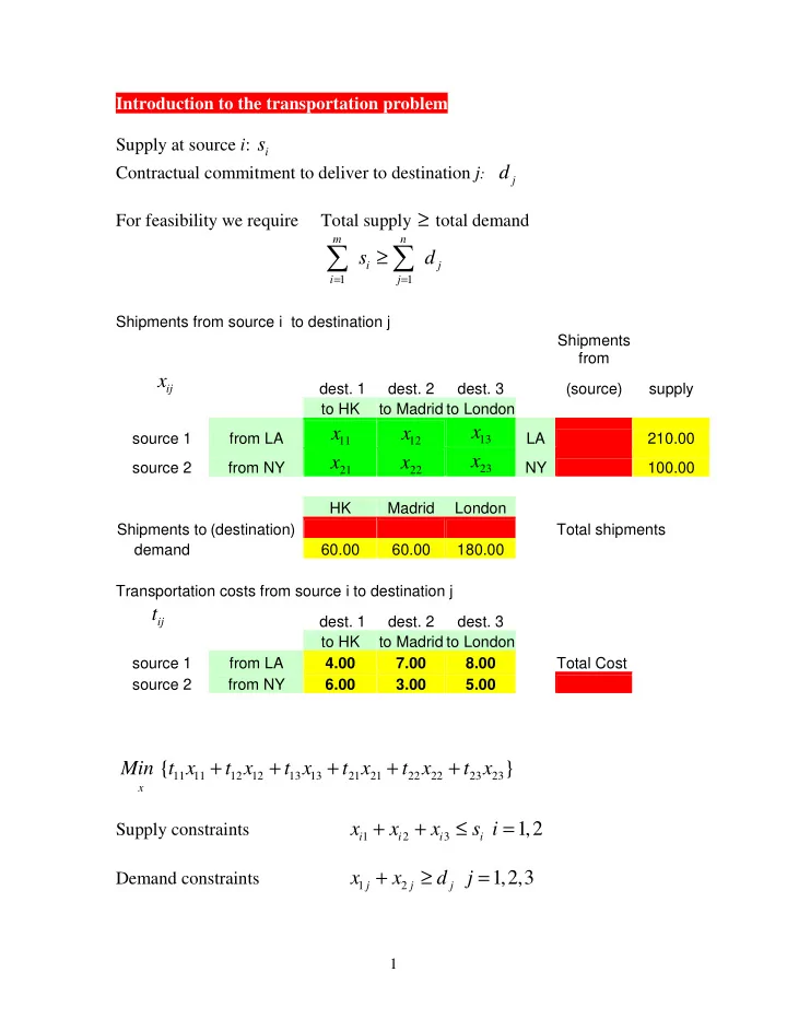
Introduction to the transportation problem s Supply at source i : i d Contractual commitment to deliver to destination j : j For feasibility we require Total supply ≥ total demand m n ≥ s d ∑ ∑ i j = = i 1 j 1 Shipments from source i to destination j Shipments from x dest. 1 dest. 2 dest. 3 (source) supply ij to HK to Madrid to London x x x source 1 from LA LA 210.00 13 11 12 x x x source 2 from NY NY 100.00 23 21 22 HK Madrid London Shipments to (destination) Total shipments demand 60.00 60.00 180.00 Transportation costs from source i to destination j t ij dest. 1 dest. 2 dest. 3 to HK to Madrid to London source 1 from LA 4.00 7.00 8.00 Total Cost source 2 from NY 6.00 3.00 5.00 + + + + + Min t x { t x t x t x t x t x } 11 11 12 12 13 13 21 21 22 22 23 23 x + + ≤ i = x x x s 1,2 Supply constraints i 1 i 2 i 3 i + ≥ j = x x d 1,2,3 Demand constraints 1 2 j j j 1

The dual problem Economic approach: Shadow prices are “as if” prices = ≤ MR MC MR MC If route ij is used , if not, ij ij ij ij θ be the price the shipper pays at source i . Let i µ be the price the shipper receives at destination j . Let j = µ = θ + MR MC t , ij j ij i ij x > µ = θ + * 0 t Thus if , then ij j i ij x = µ ≤ θ + * 0 t And if , then ij j i ij Summary: Shadow price at source + cost of shipping is at least equal to the shadow price at the destination. + + ≤ θ x x x s (LA) shadow price 11 12 13 1 1 + + ≤ θ x x x s (NY) shadow price 21 22 23 2 2 + ≥ µ x x d (HK) shadow price 11 21 1 1 + ≥ µ x x d (Madrid) shadow price 12 22 2 2 + ≥ µ x x d (London) shadow price 13 23 3 3 2

Using solver Shipments from source i to destination j x_ij destinations (source) supply d1 (HK) d2 (Madrid) d3 (London) sources s1 (LA) x_11 x_12 x_13 row sum 200.00 s2 (NY) X_21 x_22 x_23 row sum 100.00 (destination) col sum col sum col sum demand 60.00 60.00 180.00 Transportation costs from source i to destination j t_ij dest. 1 dest. 2 dest. 3 to HK to Madrid to London source 1 from LA Total Cost 4.00 7.00 8.00 source 2 from NY 6.00 3.00 5.00 T Target cell: =sumproduct(green block, yellow block) CONSTRAINTS Supply: red col <= yellow col Demand: red row >= yellow row Non-negativity: green block >= 0 Solvers printout of imputed prices. Increasing a supply lowers transportation cost so each source shadow price will be shown as negative. Increasing a demand raises transportation cost so each destination shadow price will be shown as positive. In our approach we define shadow prices as the effect on value when a constraint is relaxed so all shadow prices are non-negative 3

Selecting the initial feasible shipments: Start in the top left corner and put in the smallest number which satisfies one of the constraints with equality. Move to the next row or column and repeat. The first such step is shown below. x_ij destinations (source) supply d1 (HK) d2 (Madrid) d3 (London) * sources s1 (LA) 60 60 210.00 s2 (NY) 0 0 100.00 (destination) 60 0 0 demand 60.00 60.00 180.00 4