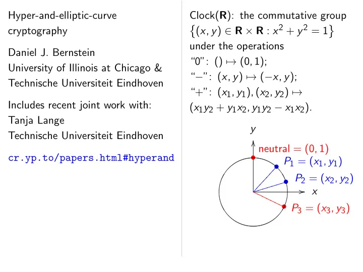
[PPT] - Hyper-and-elliptic-curve Clock( R ): the commutative group ( x; y PowerPoint Presentation

SLIDE 1

Hyper-and-elliptic-curve cryptography Daniel J. Bernstein University of Illinois at Chicago & Technische Universiteit Eindhoven Includes recent joint work with: Tanja Lange Technische Universiteit Eindhoven cr.yp.to/papers.html#hyperand Clock(R): the commutative group ˘ (x; y) ∈ R × R : x2 + y2 = 1 ¯ under the operations “0”: () → (0; 1); “−”: (x; y) → (−x; y); “+”: (x1; y1); (x2; y2) → (x1y2 + y1x2; y1y2 − x1x2). y x

neutral = (0; 1)
P1 = (x1; y1)
✂

✂ ✂ ✂ ✂ ✂ ✂ P2 = (x2; y2)

✐

✐ ✐ ✐ ✐ ✐ ✐ P3 = (x3; y3)

P

P P P P P P

SLIDE 2

er-and-elliptic-curve cryptography

J. Bernstein

University of Illinois at Chicago & echnische Universiteit Eindhoven Includes recent joint work with: Lange echnische Universiteit Eindhoven cr.yp.to/papers.html#hyperand Clock(R): the commutative group ˘ (x; y) ∈ R × R : x2 + y2 = 1 ¯ under the operations “0”: () → (0; 1); “−”: (x; y) → (−x; y); “+”: (x1; y1); (x2; y2) → (x1y2 + y1x2; y1y2 − x1x2). y x

neutral = (0; 1)
P1 = (x1; y1)
✂

✂ ✂ ✂ ✂ ✂ ✂ P2 = (x2; y2)

✐

✐ ✐ ✐ ✐ ✐ ✐ P3 = (x3; y3)

P

P P P P P P More clo “A parametrize t → (sin is a group inducing

SLIDE 3

er-and-elliptic-curve Bernstein Illinois at Chicago & Universiteit Eindhoven joint work with: Universiteit Eindhoven cr.yp.to/papers.html#hyperand Clock(R): the commutative group ˘ (x; y) ∈ R × R : x2 + y2 = 1 ¯ under the operations “0”: () → (0; 1); “−”: (x; y) → (−x; y); “+”: (x1; y1); (x2; y2) → (x1y2 + y1x2; y1y2 − x1x2). y x

neutral = (0; 1)
P1 = (x1; y1)
✂

✂ ✂ ✂ ✂ ✂ ✂ P2 = (x2; y2)

✐

✐ ✐ ✐ ✐ ✐ ✐ P3 = (x3; y3)

P

P P P P P P More clock perspectives: “A parametrized clo t → (sin t; cos t) is a group hom R inducing R=2ıZ , ։

SLIDE 4

Chicago & Eindhoven with: Eindhoven cr.yp.to/papers.html#hyperand Clock(R): the commutative group ˘ (x; y) ∈ R × R : x2 + y2 = 1 ¯ under the operations “0”: () → (0; 1); “−”: (x; y) → (−x; y); “+”: (x1; y1); (x2; y2) → (x1y2 + y1x2; y1y2 − x1x2). y x

neutral = (0; 1)
P1 = (x1; y1)
✂

✂ ✂ ✂ ✂ ✂ ✂ P2 = (x2; y2)

✐

✐ ✐ ✐ ✐ ✐ ✐ P3 = (x3; y3)

P

P P P P P P More clock perspectives: “A parametrized clock”: t → (sin t; cos t) is a group hom R ։ Clock(R inducing R=2ıZ , ։ Clock(R

SLIDE 5

Clock(R): the commutative group ˘ (x; y) ∈ R × R : x2 + y2 = 1 ¯ under the operations “0”: () → (0; 1); “−”: (x; y) → (−x; y); “+”: (x1; y1); (x2; y2) → (x1y2 + y1x2; y1y2 − x1x2). y x

neutral = (0; 1)
P1 = (x1; y1)
✂

✂ ✂ ✂ ✂ ✂ ✂ P2 = (x2; y2)

✐

✐ ✐ ✐ ✐ ✐ ✐ P3 = (x3; y3)

P

P P P P P P More clock perspectives: “A parametrized clock”: t → (sin t; cos t) is a group hom R ։ Clock(R) inducing R=2ıZ , ։ Clock(R).

SLIDE 6

Clock(R): the commutative group ˘ (x; y) ∈ R × R : x2 + y2 = 1 ¯ under the operations “0”: () → (0; 1); “−”: (x; y) → (−x; y); “+”: (x1; y1); (x2; y2) → (x1y2 + y1x2; y1y2 − x1x2). y x

neutral = (0; 1)
P1 = (x1; y1)
✂

✂ ✂ ✂ ✂ ✂ ✂ P2 = (x2; y2)

✐

✐ ✐ ✐ ✐ ✐ ✐ P3 = (x3; y3)

P

P P P P P P More clock perspectives: “A parametrized clock”: t → (sin t; cos t) is a group hom R ։ Clock(R) inducing R=2ıZ , ։ Clock(R). “Complex numbers of norm 1”: {u ∈ C : uu = 1} is a group under 1; u → u; u1; u2 → u1u2. (x; y) → y + ix is a group hom Clock(R) , ։ {u ∈ C : uu = 1}.

SLIDE 7

Clock(R): the commutative group ˘ (x; y) ∈ R × R : x2 + y2 = 1 ¯ under the operations “0”: () → (0; 1); “−”: (x; y) → (−x; y); “+”: (x1; y1); (x2; y2) → (x1y2 + y1x2; y1y2 − x1x2). y x

neutral = (0; 1)
P1 = (x1; y1)
✂

✂ ✂ ✂ ✂ ✂ ✂ P2 = (x2; y2)

✐

✐ ✐ ✐ ✐ ✐ ✐ P3 = (x3; y3)

P

P P P P P P More clock perspectives: “A parametrized clock”: t → (sin t; cos t) is a group hom R ։ Clock(R) inducing R=2ıZ , ։ Clock(R). “Complex numbers of norm 1”: {u ∈ C : uu = 1} is a group under 1; u → u; u1; u2 → u1u2. (x; y) → y + ix is a group hom Clock(R) , ։ {u ∈ C : uu = 1}. “2-dimensional rotations”: (x; y) → “ y

x −x y

” is a group hom Clock(R) , ։ SO2(R).

SLIDE 8

R): the commutative group ) ∈ R × R : x2 + y2 = 1 ¯ the operations () → (0; 1); (x; y) → (−x; y); (x1; y1); (x2; y2) → + y1x2; y1y2 − x1x2). y x

neutral = (0; 1)
P1 = (x1; y1)
✂

✂ ✂ ✂ ✂ ✂ ✂ P2 = (x2; y2)

✐

✐ ✐ ✐ ✐ ✐ ✐ P3 = (x3; y3)

P

P P P P P P More clock perspectives: “A parametrized clock”: t → (sin t; cos t) is a group hom R ։ Clock(R) inducing R=2ıZ , ։ Clock(R). “Complex numbers of norm 1”: {u ∈ C : uu = 1} is a group under 1; u → u; u1; u2 → u1u2. (x; y) → y + ix is a group hom Clock(R) , ։ {u ∈ C : uu = 1}. “2-dimensional rotations”: (x; y) → “ y

x −x y

” is a group hom Clock(R) , ։ SO2(R). Clocks over Clock(F7 ˘ (x; y) ∈ Group op · · · · · · · Diagram −3; −2; −

SLIDE 9

commutative group : x2 + y2 = 1 ¯ erations 1); −x; y);

2; y2) →

y2 − x1x2). x

neutral = (0; 1)

P1 = (x1; y1)

✂

✂ P2 = (x2; y2)

✐

✐ ✐ ✐ P3 = (x3; y3)

P

P P More clock perspectives: “A parametrized clock”: t → (sin t; cos t) is a group hom R ։ Clock(R) inducing R=2ıZ , ։ Clock(R). “Complex numbers of norm 1”: {u ∈ C : uu = 1} is a group under 1; u → u; u1; u2 → u1u2. (x; y) → y + ix is a group hom Clock(R) , ։ {u ∈ C : uu = 1}. “2-dimensional rotations”: (x; y) → “ y

x −x y

” is a group hom Clock(R) , ։ SO2(R). Clocks over finite fields Clock(F7) = ˘ (x; y) ∈ F7 × F7 Group operations as · · · · · · · · · · · · · · · · · · · · · · · · · · · ·

Diagram plots F7 as

−3; −2; −1; 0; 1; 2;

SLIDE 10

commutative group = 1 ¯ ). x (0; 1) (x1; y1) = (x2; y2) (x3; y3) More clock perspectives: “A parametrized clock”: t → (sin t; cos t) is a group hom R ։ Clock(R) inducing R=2ıZ , ։ Clock(R). “Complex numbers of norm 1”: {u ∈ C : uu = 1} is a group under 1; u → u; u1; u2 → u1u2. (x; y) → y + ix is a group hom Clock(R) , ։ {u ∈ C : uu = 1}. “2-dimensional rotations”: (x; y) → “ y

x −x y

” is a group hom Clock(R) , ։ SO2(R). Clocks over finite fields Clock(F7) = ˘ (x; y) ∈ F7 × F7 : x2 + y2 Group operations as before. · · · · · · · · · · · · · · · · · · · · · · · · · · · · · · · · · · · · · · · · · · · · · · · · ·

Diagram plots F7 as

−3; −2; −1; 0; 1; 2; 3.

SLIDE 11

More clock perspectives: “A parametrized clock”: t → (sin t; cos t) is a group hom R ։ Clock(R) inducing R=2ıZ , ։ Clock(R). “Complex numbers of norm 1”: {u ∈ C : uu = 1} is a group under 1; u → u; u1; u2 → u1u2. (x; y) → y + ix is a group hom Clock(R) , ։ {u ∈ C : uu = 1}. “2-dimensional rotations”: (x; y) → “ y

x −x y

” is a group hom Clock(R) , ։ SO2(R). Clocks over finite fields Clock(F7) = ˘ (x; y) ∈ F7 × F7 : x2 + y2 = 1 ¯ . Group operations as before. · · · · · · · · · · · · · · · · · · · · · · · · · · · · · · · · · · · · · · · · · · · · · · · · ·

Diagram plots F7 as

−3; −2; −1; 0; 1; 2; 3.

SLIDE 12

clock perspectives: rametrized clock”: (sin t; cos t) group hom R ։ Clock(R) inducing R=2ıZ , ։ Clock(R). “Complex numbers of norm 1”: : uu = 1} is a group under u; u1; u2 → u1u2. → y + ix is a group hom R) , ։ {u ∈ C : uu = 1}. “2-dimensional rotations”: → “ y

x −x y

” is a hom Clock(R) , ։ SO2(R). Clocks over finite fields Clock(F7) = ˘ (x; y) ∈ F7 × F7 : x2 + y2 = 1 ¯ . Group operations as before. · · · · · · · · · · · · · · · · · · · · · · · · · · · · · · · · · · · · · · · · · · · · · · · · ·

Diagram plots F7 as

−3; −2; −1; 0; 1; 2; 3. Larger exa Examples in Clock( 2(1000; 2)

SLIDE 13

rspectives: clock”: R ։ Clock(R) , ։ Clock(R). ers of norm 1”: } is a group under → u1u2. is a group hom ∈ C : uu = 1}. rotations”: ” is a ck(R) , ։ SO2(R). Clocks over finite fields Clock(F7) = ˘ (x; y) ∈ F7 × F7 : x2 + y2 = 1 ¯ . Group operations as before. · · · · · · · · · · · · · · · · · · · · · · · · · · · · · · · · · · · · · · · · · · · · · · · · ·

Diagram plots F7 as

−3; −2; −1; 0; 1; 2; 3. Larger example: Clo Examples of addition in Clock(F1000003): 2(1000; 2) = (4000

SLIDE 14

ck(R) ck(R). rm 1”: p under hom 1}. SO2(R). Clocks over finite fields Clock(F7) = ˘ (x; y) ∈ F7 × F7 : x2 + y2 = 1 ¯ . Group operations as before. · · · · · · · · · · · · · · · · · · · · · · · · · · · · · · · · · · · · · · · · · · · · · · · · ·

Diagram plots F7 as

−3; −2; −1; 0; 1; 2; 3. Larger example: Clock(F1000003 Examples of addition in Clock(F1000003): 2(1000; 2) = (4000; 7).

SLIDE 15

Clocks over finite fields Clock(F7) = ˘ (x; y) ∈ F7 × F7 : x2 + y2 = 1 ¯ . Group operations as before. · · · · · · · · · · · · · · · · · · · · · · · · · · · · · · · · · · · · · · · · · · · · · · · · ·

Diagram plots F7 as

−3; −2; −1; 0; 1; 2; 3. Larger example: Clock(F1000003). Examples of addition in Clock(F1000003): 2(1000; 2) = (4000; 7).

SLIDE 16

Clocks over finite fields Clock(F7) = ˘ (x; y) ∈ F7 × F7 : x2 + y2 = 1 ¯ . Group operations as before. · · · · · · · · · · · · · · · · · · · · · · · · · · · · · · · · · · · · · · · · · · · · · · · · ·

Diagram plots F7 as

−3; −2; −1; 0; 1; 2; 3. Larger example: Clock(F1000003). Examples of addition in Clock(F1000003): 2(1000; 2) = (4000; 7). 4(1000; 2) = (56000; 97).

SLIDE 17

Clocks over finite fields Clock(F7) = ˘ (x; y) ∈ F7 × F7 : x2 + y2 = 1 ¯ . Group operations as before. · · · · · · · · · · · · · · · · · · · · · · · · · · · · · · · · · · · · · · · · · · · · · · · · ·

Diagram plots F7 as

−3; −2; −1; 0; 1; 2; 3. Larger example: Clock(F1000003). Examples of addition in Clock(F1000003): 2(1000; 2) = (4000; 7). 4(1000; 2) = (56000; 97). 8(1000; 2) = (863970; 18817).

SLIDE 18

Clocks over finite fields Clock(F7) = ˘ (x; y) ∈ F7 × F7 : x2 + y2 = 1 ¯ . Group operations as before. · · · · · · · · · · · · · · · · · · · · · · · · · · · · · · · · · · · · · · · · · · · · · · · · ·

Diagram plots F7 as

−3; −2; −1; 0; 1; 2; 3. Larger example: Clock(F1000003). Examples of addition in Clock(F1000003): 2(1000; 2) = (4000; 7). 4(1000; 2) = (56000; 97). 8(1000; 2) = (863970; 18817). 16(1000; 2) = (549438; 156853).

SLIDE 19

Clocks over finite fields Clock(F7) = ˘ (x; y) ∈ F7 × F7 : x2 + y2 = 1 ¯ . Group operations as before. · · · · · · · · · · · · · · · · · · · · · · · · · · · · · · · · · · · · · · · · · · · · · · · · ·

Diagram plots F7 as

−3; −2; −1; 0; 1; 2; 3. Larger example: Clock(F1000003). Examples of addition in Clock(F1000003): 2(1000; 2) = (4000; 7). 4(1000; 2) = (56000; 97). 8(1000; 2) = (863970; 18817). 16(1000; 2) = (549438; 156853). 17(1000; 2) = (951405; 877356).

SLIDE 20

Clocks over finite fields Clock(F7) = ˘ (x; y) ∈ F7 × F7 : x2 + y2 = 1 ¯ . Group operations as before. · · · · · · · · · · · · · · · · · · · · · · · · · · · · · · · · · · · · · · · · · · · · · · · · ·

Diagram plots F7 as

−3; −2; −1; 0; 1; 2; 3. Larger example: Clock(F1000003). Examples of addition in Clock(F1000003): 2(1000; 2) = (4000; 7). 4(1000; 2) = (56000; 97). 8(1000; 2) = (863970; 18817). 16(1000; 2) = (549438; 156853). 17(1000; 2) = (951405; 877356). “Scalar multiplication” maps Z × Clock(Fq) → Clock(Fq) by n; P → nP. We’ll build cryptography from scalar multiplication.

SLIDE 21

ver finite fields

F7) = ) ∈ F7 × F7 : x2 + y2 = 1 ¯ .

perations as before.

· · · · · · · · · · · · · · · · · · · · · · · · · · · · · · · · · · · · · · · · · · · · · · · · ·

Diagram plots F7 as

2; −1; 0; 1; 2; 3. Larger example: Clock(F1000003). Examples of addition in Clock(F1000003): 2(1000; 2) = (4000; 7). 4(1000; 2) = (56000; 97). 8(1000; 2) = (863970; 18817). 16(1000; 2) = (549438; 156853). 17(1000; 2) = (951405; 877356). “Scalar multiplication” maps Z × Clock(Fq) → Clock(Fq) by n; P → nP. We’ll build cryptography from scalar multiplication. A fast metho take 0 if negate ( double (n add P to else subtract

SLIDE 22

ite fields

7 : x2 + y2 = 1

¯ . erations as before. · · · · · · · · · · · · · · · · · · · · · · · · · · · ·

7 as

; 2; 3. Larger example: Clock(F1000003). Examples of addition in Clock(F1000003): 2(1000; 2) = (4000; 7). 4(1000; 2) = (56000; 97). 8(1000; 2) = (863970; 18817). 16(1000; 2) = (549438; 156853). 17(1000; 2) = (951405; 877356). “Scalar multiplication” maps Z × Clock(Fq) → Clock(Fq) by n; P → nP. We’ll build cryptography from scalar multiplication. A fast method to compute take 0 if n = 0; negate (−n)P if n double (n=2)P if n add P to (n − 1)P else subtract P from

SLIDE 23

2 = 1

¯ . e. · · · · · · · Larger example: Clock(F1000003). Examples of addition in Clock(F1000003): 2(1000; 2) = (4000; 7). 4(1000; 2) = (56000; 97). 8(1000; 2) = (863970; 18817). 16(1000; 2) = (549438; 156853). 17(1000; 2) = (951405; 877356). “Scalar multiplication” maps Z × Clock(Fq) → Clock(Fq) by n; P → nP. We’ll build cryptography from scalar multiplication. A fast method to compute n take 0 if n = 0; negate (−n)P if n < 0; double (n=2)P if n ∈ 2Z; add P to (n − 1)P if n − 1 ∈ else subtract P from (n + 1)

SLIDE 24

Larger example: Clock(F1000003). Examples of addition in Clock(F1000003): 2(1000; 2) = (4000; 7). 4(1000; 2) = (56000; 97). 8(1000; 2) = (863970; 18817). 16(1000; 2) = (549438; 156853). 17(1000; 2) = (951405; 877356). “Scalar multiplication” maps Z × Clock(Fq) → Clock(Fq) by n; P → nP. We’ll build cryptography from scalar multiplication. A fast method to compute nP: take 0 if n = 0; negate (−n)P if n < 0; double (n=2)P if n ∈ 2Z; add P to (n − 1)P if n − 1 ∈ 4Z; else subtract P from (n + 1)P.

SLIDE 25

Larger example: Clock(F1000003). Examples of addition in Clock(F1000003): 2(1000; 2) = (4000; 7). 4(1000; 2) = (56000; 97). 8(1000; 2) = (863970; 18817). 16(1000; 2) = (549438; 156853). 17(1000; 2) = (951405; 877356). “Scalar multiplication” maps Z × Clock(Fq) → Clock(Fq) by n; P → nP. We’ll build cryptography from scalar multiplication. A fast method to compute nP: take 0 if n = 0; negate (−n)P if n < 0; double (n=2)P if n ∈ 2Z; add P to (n − 1)P if n − 1 ∈ 4Z; else subtract P from (n + 1)P. But figuring out n given P and nP is much more difficult. 30 clock additions produce n(1000; 2) = (947472; 736284) for some 6-digit n. Can you figure out n?

SLIDE 26

example: Clock(F1000003). Examples of addition ck(F1000003): ; 2) = (4000; 7). ; 2) = (56000; 97). ; 2) = (863970; 18817). 16(1000; 2) = (549438; 156853). 17(1000; 2) = (951405; 877356). r multiplication” maps Clock(Fq) → Clock(Fq) → nP. build cryptography scalar multiplication. A fast method to compute nP: take 0 if n = 0; negate (−n)P if n < 0; double (n=2)P if n ∈ 2Z; add P to (n − 1)P if n − 1 ∈ 4Z; else subtract P from (n + 1)P. But figuring out n given P and nP is much more difficult. 30 clock additions produce n(1000; 2) = (947472; 736284) for some 6-digit n. Can you figure out n? Clock cryptography Standardize and (x; y

f large p

Alice cho Computes Bob cho Computes Alice computes Bob computes They use to encrypt

SLIDE 27

Clock(F1000003). addition

1000003):

(4000; 7). (56000; 97). (863970; 18817). (549438; 156853). (951405; 877356). multiplication” maps Clock(Fq) cryptography multiplication. A fast method to compute nP: take 0 if n = 0; negate (−n)P if n < 0; double (n=2)P if n ∈ 2Z; add P to (n − 1)P if n − 1 ∈ 4Z; else subtract P from (n + 1)P. But figuring out n given P and nP is much more difficult. 30 clock additions produce n(1000; 2) = (947472; 736284) for some 6-digit n. Can you figure out n? Clock cryptography Standardize odd prime and (x; y) ∈ Clock(

f large prime orde

Alice chooses big secret Computes her public Bob chooses big secret Computes his public Alice computes a(b Bob computes b(a They use this shared to encrypt with “AES-GCM”

SLIDE 28

1000003).

18817). 156853). 877356). maps

q)

A fast method to compute nP: take 0 if n = 0; negate (−n)P if n < 0; double (n=2)P if n ∈ 2Z; add P to (n − 1)P if n − 1 ∈ 4Z; else subtract P from (n + 1)P. But figuring out n given P and nP is much more difficult. 30 clock additions produce n(1000; 2) = (947472; 736284) for some 6-digit n. Can you figure out n? Clock cryptography Standardize odd prime power and (x; y) ∈ Clock(Fq)

f large prime order.

Alice chooses big secret a. Computes her public key a(x Bob chooses big secret b. Computes his public key b(x Alice computes a(b(x; y)). Bob computes b(a(x; y)). They use this shared secret to encrypt with “AES-GCM”

SLIDE 29

A fast method to compute nP: take 0 if n = 0; negate (−n)P if n < 0; double (n=2)P if n ∈ 2Z; add P to (n − 1)P if n − 1 ∈ 4Z; else subtract P from (n + 1)P. But figuring out n given P and nP is much more difficult. 30 clock additions produce n(1000; 2) = (947472; 736284) for some 6-digit n. Can you figure out n? Clock cryptography Standardize odd prime power q and (x; y) ∈ Clock(Fq)

f large prime order.

Alice chooses big secret a. Computes her public key a(x; y). Bob chooses big secret b. Computes his public key b(x; y). Alice computes a(b(x; y)). Bob computes b(a(x; y)). They use this shared secret to encrypt with “AES-GCM” etc.

SLIDE 30

method to compute nP: if n = 0; (−n)P if n < 0; (n=2)P if n ∈ 2Z; to (n − 1)P if n − 1 ∈ 4Z; subtract P from (n + 1)P. figuring out n P and nP much more difficult. ck additions produce ; 2) = (947472; 736284)

me 6-digit n.
u figure out n?

Clock cryptography Standardize odd prime power q and (x; y) ∈ Clock(Fq)

f large prime order.

Alice chooses big secret a. Computes her public key a(x; y). Bob chooses big secret b. Computes his public key b(x; y). Alice computes a(b(x; y)). Bob computes b(a(x; y)). They use this shared secret to encrypt with “AES-GCM” etc. Alice’s secret

Alice’s

public a(x; {Alice; Bob shared ab(x

SLIDE 31

to compute nP: n < 0; if n ∈ 2Z; 1)P if n − 1 ∈ 4Z; from (n + 1)P. n difficult. additions produce (947472; 736284) n.

ut n?

Clock cryptography Standardize odd prime power q and (x; y) ∈ Clock(Fq)

f large prime order.

Alice chooses big secret a. Computes her public key a(x; y). Bob chooses big secret b. Computes his public key b(x; y). Alice computes a(b(x; y)). Bob computes b(a(x; y)). They use this shared secret to encrypt with “AES-GCM” etc. Alice’s secret key a

Alice’s

public key a(x; y) ▲ ▲ ▲ ▲ ▲ ▲ rrrr {Alice; Bob}’s shared secret ab(x; y) =

SLIDE 32

nP: 1 ∈ 4Z; 1)P. duce 736284) Clock cryptography Standardize odd prime power q and (x; y) ∈ Clock(Fq)

f large prime order.

Alice chooses big secret a. Computes her public key a(x; y). Bob chooses big secret b. Computes his public key b(x; y). Alice computes a(b(x; y)). Bob computes b(a(x; y)). They use this shared secret to encrypt with “AES-GCM” etc. Alice’s secret key a

Bob’s

secret k

Alice’s

public key a(x; y)

▲

▲ ▲ ▲ ▲ ▲ ▲ Bob’s public b(x; y rrrrrrr {Alice; Bob}’s shared secret ab(x; y) = {Bob; Alice shared s ba(x;

SLIDE 33

Clock cryptography Standardize odd prime power q and (x; y) ∈ Clock(Fq)

f large prime order.

Alice chooses big secret a. Computes her public key a(x; y). Bob chooses big secret b. Computes his public key b(x; y). Alice computes a(b(x; y)). Bob computes b(a(x; y)). They use this shared secret to encrypt with “AES-GCM” etc. Alice’s secret key a

Bob’s

secret key b

Alice’s

public key a(x; y)

▲

▲ ▲ ▲ ▲ ▲ ▲ Bob’s public key b(x; y) rrrrrrr {Alice; Bob}’s shared secret ab(x; y) = {Bob; Alice}’s shared secret ba(x; y)

SLIDE 34

Clock cryptography Standardize odd prime power q and (x; y) ∈ Clock(Fq)

f large prime order.

Alice chooses big secret a. Computes her public key a(x; y). Bob chooses big secret b. Computes his public key b(x; y). Alice computes a(b(x; y)). Bob computes b(a(x; y)). They use this shared secret to encrypt with “AES-GCM” etc. Alice’s secret key a

Bob’s

secret key b

Alice’s

public key a(x; y)

▲

▲ ▲ ▲ ▲ ▲ ▲ Bob’s public key b(x; y) rrrrrrr {Alice; Bob}’s shared secret ab(x; y) = {Bob; Alice}’s shared secret ba(x; y) Need surprisingly large q to avoid state-of-the-art attacks. Recommendation: q > 21500. Better: Switch to elliptic curves.

SLIDE 35

cryptography Standardize odd prime power q ; y) ∈ Clock(Fq) rge prime order. chooses big secret a. Computes her public key a(x; y). chooses big secret b. Computes his public key b(x; y). computes a(b(x; y)). computes b(a(x; y)). use this shared secret encrypt with “AES-GCM” etc. Alice’s secret key a

Bob’s

secret key b

Alice’s

public key a(x; y)

▲

▲ ▲ ▲ ▲ ▲ ▲ Bob’s public key b(x; y) rrrrrrr {Alice; Bob}’s shared secret ab(x; y) = {Bob; Alice}’s shared secret ba(x; y) Need surprisingly large q to avoid state-of-the-art attacks. Recommendation: q > 21500. Better: Switch to elliptic curves. Addition x2 + y2 Sum of ( ((x1y2+y (y1y2−x

SLIDE 36

cryptography prime power q ck(Fq) rder. big secret a. public key a(x; y). secret b. public key b(x; y). a(b(x; y)). (a(x; y)). shared secret “AES-GCM” etc. Alice’s secret key a

Bob’s

secret key b

Alice’s

public key a(x; y)

▲

▲ ▲ ▲ ▲ ▲ ▲ Bob’s public key b(x; y) rrrrrrr {Alice; Bob}’s shared secret ab(x; y) = {Bob; Alice}’s shared secret ba(x; y) Need surprisingly large q to avoid state-of-the-art attacks. Recommendation: q > 21500. Better: Switch to elliptic curves. Addition on an elliptic y

neutral
P
☞

☞ ☞ ☞ ❢ ❢ ❢ ❢ ❬ ❬ ❬ ❬ x2 + y2 = 1 − 30x Sum of (x1; y1) and ((x1y2+y1x2)=(1− (y1y2−x1x2)=(1+30

SLIDE 37

wer q . (x; y). (x; y). )). cret “AES-GCM” etc. Alice’s secret key a

Bob’s

secret key b

Alice’s

public key a(x; y)

▲

▲ ▲ ▲ ▲ ▲ ▲ Bob’s public key b(x; y) rrrrrrr {Alice; Bob}’s shared secret ab(x; y) = {Bob; Alice}’s shared secret ba(x; y) Need surprisingly large q to avoid state-of-the-art attacks. Recommendation: q > 21500. Better: Switch to elliptic curves. Addition on an elliptic curve y x

neutral = (0;
P1 = (x1; y
☞

☞ ☞ ☞ P2 = (x

❢

❢ ❢ ❢ ❢ P3 = (

❬

❬ ❬ ❬ ❬ ❬ x2 + y2 = 1 − 30x2y2. Sum of (x1; y1) and (x2; y2) ((x1y2+y1x2)=(1−30x1x2y1y (y1y2−x1x2)=(1+30x1x2y1y

SLIDE 38

Alice’s secret key a

Bob’s

secret key b

Alice’s

public key a(x; y)

▲

▲ ▲ ▲ ▲ ▲ ▲ Bob’s public key b(x; y) rrrrrrr {Alice; Bob}’s shared secret ab(x; y) = {Bob; Alice}’s shared secret ba(x; y) Need surprisingly large q to avoid state-of-the-art attacks. Recommendation: q > 21500. Better: Switch to elliptic curves. Addition on an elliptic curve y x

neutral = (0; 1)
P1 = (x1; y1)
☞

☞ ☞ ☞ P2 = (x2; y2)

❢

❢ ❢ ❢ ❢ P3 = (x3; y3)

❬

❬ ❬ ❬ ❬ ❬ x2 + y2 = 1 − 30x2y2. Sum of (x1; y1) and (x2; y2) is ((x1y2+y1x2)=(1−30x1x2y1y2), (y1y2−x1x2)=(1+30x1x2y1y2)).

SLIDE 39

Alice’s secret key a

Bob’s

secret key b

Alice’s

public key x; y)

▲

▲ ▲ ▲ ▲ ▲ ▲ Bob’s public key b(x; y) rrrrrrr Alice; Bob}’s red secret (x; y) = {Bob; Alice}’s shared secret ba(x; y) surprisingly large q avoid state-of-the-art attacks. Recommendation: q > 21500. Better: Switch to elliptic curves. Addition on an elliptic curve y x

neutral = (0; 1)
P1 = (x1; y1)
☞

☞ ☞ ☞ P2 = (x2; y2)

❢

❢ ❢ ❢ ❢ P3 = (x3; y3)

❬

❬ ❬ ❬ ❬ ❬ x2 + y2 = 1 − 30x2y2. Sum of (x1; y1) and (x2; y2) is ((x1y2+y1x2)=(1−30x1x2y1y2), (y1y2−x1x2)=(1+30x1x2y1y2)). The clock x2 + y2 Sum of ( (x1y2 + y y1y2 − x

SLIDE 40

Bob’s secret key b

▲

▲ ▲ Bob’s public key b(x; y) rrrr = {Bob; Alice}’s shared secret ba(x; y) risingly large q state-of-the-art attacks. Recommendation: q > 21500. to elliptic curves. Addition on an elliptic curve y x

neutral = (0; 1)
P1 = (x1; y1)
☞

☞ ☞ ☞ P2 = (x2; y2)

❢

❢ ❢ ❢ ❢ P3 = (x3; y3)

❬

❬ ❬ ❬ ❬ ❬ x2 + y2 = 1 − 30x2y2. Sum of (x1; y1) and (x2; y2) is ((x1y2+y1x2)=(1−30x1x2y1y2), (y1y2−x1x2)=(1+30x1x2y1y2)). The clock again, fo y

neutral
✂

✂ ✂ ✂ ✂ ✂ ✐ ✐ ✐ ✐ ✐ P P P P P x2 + y2 = 1. Sum of (x1; y1) and (x1y2 + y1x2, y1y2 − x1x2).

SLIDE 41

Bob’s secret key b

Bob’s

public key ; y) Alice}’s secret x; y) attacks.

1500.

curves. Addition on an elliptic curve y x

neutral = (0; 1)
P1 = (x1; y1)
☞

☞ ☞ ☞ P2 = (x2; y2)

❢

❢ ❢ ❢ ❢ P3 = (x3; y3)

❬

❬ ❬ ❬ ❬ ❬ x2 + y2 = 1 − 30x2y2. Sum of (x1; y1) and (x2; y2) is ((x1y2+y1x2)=(1−30x1x2y1y2), (y1y2−x1x2)=(1+30x1x2y1y2)). The clock again, for comparison: y x

neutral = (0;
P1 = (x
✂

✂ ✂ ✂ ✂ ✂ ✂ P2 =

✐

✐ ✐ ✐ ✐ ✐ ✐ P3 = (

P

P P P P P P x2 + y2 = 1. Sum of (x1; y1) and (x2; y2) (x1y2 + y1x2, y1y2 − x1x2).

SLIDE 42

Addition on an elliptic curve y x

neutral = (0; 1)
P1 = (x1; y1)
☞

☞ ☞ ☞ P2 = (x2; y2)

❢

❢ ❢ ❢ ❢ P3 = (x3; y3)

❬

❬ ❬ ❬ ❬ ❬ x2 + y2 = 1 − 30x2y2. Sum of (x1; y1) and (x2; y2) is ((x1y2+y1x2)=(1−30x1x2y1y2), (y1y2−x1x2)=(1+30x1x2y1y2)). The clock again, for comparison: y x

neutral = (0; 1)
P1 = (x1; y1)
✂

✂ ✂ ✂ ✂ ✂ ✂ P2 = (x2; y2)

✐

✐ ✐ ✐ ✐ ✐ ✐ P3 = (x3; y3)

P

P P P P P P x2 + y2 = 1. Sum of (x1; y1) and (x2; y2) is (x1y2 + y1x2, y1y2 − x1x2).

SLIDE 43

Addition on an elliptic curve y x

neutral = (0; 1)
P1 = (x1; y1)
☞

☞ ☞ ☞ P2 = (x2; y2)

❢

❢ ❢ ❢ ❢ P3 = (x3; y3)

❬

❬ ❬ ❬ ❬ ❬

2 = 1 − 30x2y2.

f (x1; y1) and (x2; y2) is

+y1x2)=(1−30x1x2y1y2), −x1x2)=(1+30x1x2y1y2)). The clock again, for comparison: y x

neutral = (0; 1)
P1 = (x1; y1)
✂

✂ ✂ ✂ ✂ ✂ ✂ P2 = (x2; y2)

✐

✐ ✐ ✐ ✐ ✐ ✐ P3 = (x3; y3)

P

P P P P P P x2 + y2 = 1. Sum of (x1; y1) and (x2; y2) is (x1y2 + y1x2, y1y2 − x1x2). More elliptic Choose an Choose a {(x; y) ∈ x2 + is a “complete “The Edw (x1; y1) + where x3 = x1 1 + y3 = y1 1 −

SLIDE 44

elliptic curve x

neutral = (0; 1)

P1 = (x1; y1)

P2 = (x2; y2)
❢

❢ P3 = (x3; y3)

❬

❬ ❬ 30x2y2. and (x2; y2) is −30x1x2y1y2), (1+30x1x2y1y2)). The clock again, for comparison: y x

neutral = (0; 1)
P1 = (x1; y1)
✂

✂ ✂ ✂ ✂ ✂ ✂ P2 = (x2; y2)

✐

✐ ✐ ✐ ✐ ✐ ✐ P3 = (x3; y3)

P

P P P P P P x2 + y2 = 1. Sum of (x1; y1) and (x2; y2) is (x1y2 + y1x2, y1y2 − x1x2). More elliptic curves Choose an odd prime Choose a non-squa {(x; y) ∈ Fq × Fq x2 + y2 = 1 + is a “complete Edw “The Edwards addition (x1; y1) + (x2; y2) = where x3 = x1y2 + y1x2 1 + dx1x2y1y y3 = y1y2 − x1x2 1 − dx1x2y1y

SLIDE 45

curve x (0; 1) ; y1) (x2; y2) (x3; y3) ) is

1y2), 1y2)).

The clock again, for comparison: y x

neutral = (0; 1)
P1 = (x1; y1)
✂

✂ ✂ ✂ ✂ ✂ ✂ P2 = (x2; y2)

✐

✐ ✐ ✐ ✐ ✐ ✐ P3 = (x3; y3)

P

P P P P P P x2 + y2 = 1. Sum of (x1; y1) and (x2; y2) is (x1y2 + y1x2, y1y2 − x1x2). More elliptic curves Choose an odd prime power Choose a non-square d ∈ Fq {(x; y) ∈ Fq × Fq : x2 + y2 = 1 + dx2y2} is a “complete Edwards curve”. “The Edwards addition law”: (x1; y1) + (x2; y2) = (x3; y3) where x3 = x1y2 + y1x2 1 + dx1x2y1y2 , y3 = y1y2 − x1x2 1 − dx1x2y1y2 .

SLIDE 46

The clock again, for comparison: y x

neutral = (0; 1)
P1 = (x1; y1)
✂

✂ ✂ ✂ ✂ ✂ ✂ P2 = (x2; y2)

✐

✐ ✐ ✐ ✐ ✐ ✐ P3 = (x3; y3)

P

P P P P P P x2 + y2 = 1. Sum of (x1; y1) and (x2; y2) is (x1y2 + y1x2, y1y2 − x1x2). More elliptic curves Choose an odd prime power q. Choose a non-square d ∈ Fq. {(x; y) ∈ Fq × Fq : x2 + y2 = 1 + dx2y2} is a “complete Edwards curve”. “The Edwards addition law”: (x1; y1) + (x2; y2) = (x3; y3) where x3 = x1y2 + y1x2 1 + dx1x2y1y2 , y3 = y1y2 − x1x2 1 − dx1x2y1y2 .

SLIDE 47

clock again, for comparison: y x

neutral = (0; 1)
P1 = (x1; y1)
✂

✂ ✂ ✂ ✂ ✂ ✂ P2 = (x2; y2)

✐

✐ ✐ ✐ ✐ ✐ ✐ P3 = (x3; y3)

P

P P P P P P

2 = 1.

f (x1; y1) and (x2; y2) is

+ y1x2, − x1x2). More elliptic curves Choose an odd prime power q. Choose a non-square d ∈ Fq. {(x; y) ∈ Fq × Fq : x2 + y2 = 1 + dx2y2} is a “complete Edwards curve”. “The Edwards addition law”: (x1; y1) + (x2; y2) = (x3; y3) where x3 = x1y2 + y1x2 1 + dx1x2y1y2 , y3 = y1y2 − x1x2 1 − dx1x2y1y2 . “What if

SLIDE 48

again, for comparison: x

neutral = (0; 1)

P1 = (x1; y1)

✂

✂ P2 = (x2; y2)

✐

✐ ✐ ✐ P3 = (x3; y3)

P

P P and (x2; y2) is More elliptic curves Choose an odd prime power q. Choose a non-square d ∈ Fq. {(x; y) ∈ Fq × Fq : x2 + y2 = 1 + dx2y2} is a “complete Edwards curve”. “The Edwards addition law”: (x1; y1) + (x2; y2) = (x3; y3) where x3 = x1y2 + y1x2 1 + dx1x2y1y2 , y3 = y1y2 − x1x2 1 − dx1x2y1y2 . “What if denominato

SLIDE 49

comparison: x (0; 1) (x1; y1) = (x2; y2) (x3; y3) ) is More elliptic curves Choose an odd prime power q. Choose a non-square d ∈ Fq. {(x; y) ∈ Fq × Fq : x2 + y2 = 1 + dx2y2} is a “complete Edwards curve”. “The Edwards addition law”: (x1; y1) + (x2; y2) = (x3; y3) where x3 = x1y2 + y1x2 1 + dx1x2y1y2 , y3 = y1y2 − x1x2 1 − dx1x2y1y2 . “What if denominators are 0?”

SLIDE 50

More elliptic curves Choose an odd prime power q. Choose a non-square d ∈ Fq. {(x; y) ∈ Fq × Fq : x2 + y2 = 1 + dx2y2} is a “complete Edwards curve”. “The Edwards addition law”: (x1; y1) + (x2; y2) = (x3; y3) where x3 = x1y2 + y1x2 1 + dx1x2y1y2 , y3 = y1y2 − x1x2 1 − dx1x2y1y2 . “What if denominators are 0?”

SLIDE 51

More elliptic curves Choose an odd prime power q. Choose a non-square d ∈ Fq. {(x; y) ∈ Fq × Fq : x2 + y2 = 1 + dx2y2} is a “complete Edwards curve”. “The Edwards addition law”: (x1; y1) + (x2; y2) = (x3; y3) where x3 = x1y2 + y1x2 1 + dx1x2y1y2 , y3 = y1y2 − x1x2 1 − dx1x2y1y2 . “What if denominators are 0?” Answer: They aren’t! If x2

1 + y2 1 = 1 + dx2 1y2 1

and x2

2 + y2 2 = 1 + dx2 2y2 2

then dx1x2y1y2 can’t be ±1.

SLIDE 52

More elliptic curves Choose an odd prime power q. Choose a non-square d ∈ Fq. {(x; y) ∈ Fq × Fq : x2 + y2 = 1 + dx2y2} is a “complete Edwards curve”. “The Edwards addition law”: (x1; y1) + (x2; y2) = (x3; y3) where x3 = x1y2 + y1x2 1 + dx1x2y1y2 , y3 = y1y2 − x1x2 1 − dx1x2y1y2 . “What if denominators are 0?” Answer: They aren’t! If x2

1 + y2 1 = 1 + dx2 1y2 1

and x2

2 + y2 2 = 1 + dx2 2y2 2

then dx1x2y1y2 can’t be ±1. Main steps in proof: If (dx1x2y1y2)2 = 1 then curve equation implies (x1 + dx1x2y1y2y1)2 = dx2

1y2 1 (x2 + y2)2.

Conclude that d is a square. But d is not a square! Q.E.D.

SLIDE 53

elliptic curves

se an odd prime power q.
se a non-square d ∈ Fq.

) ∈ Fq × Fq : + y2 = 1 + dx2y2} “complete Edwards curve”. Edwards addition law”: ) + (x2; y2) = (x3; y3) x1y2 + y1x2 + dx1x2y1y2 , y1y2 − x1x2 − dx1x2y1y2 . “What if denominators are 0?” Answer: They aren’t! If x2

1 + y2 1 = 1 + dx2 1y2 1

and x2

2 + y2 2 = 1 + dx2 2y2 2

then dx1x2y1y2 can’t be ±1. Main steps in proof: If (dx1x2y1y2)2 = 1 then curve equation implies (x1 + dx1x2y1y2y1)2 = dx2

1y2 1 (x2 + y2)2.

Conclude that d is a square. But d is not a square! Q.E.D. “Doesn’t standard e.g. “Every is linear.” e.g. “Theo cardinalit

f addition

two.” (1995

SLIDE 54

curves rime power q. non-square d ∈ Fq.

q :

1 + dx2y2} Edwards curve”. addition law”: ) = (x3; y3) x2

1y2

, x2

1y2

. “What if denominators are 0?” Answer: They aren’t! If x2

1 + y2 1 = 1 + dx2 1y2 1

and x2

2 + y2 2 = 1 + dx2 2y2 2

then dx1x2y1y2 can’t be ±1. Main steps in proof: If (dx1x2y1y2)2 = 1 then curve equation implies (x1 + dx1x2y1y2y1)2 = dx2

1y2 1 (x2 + y2)2.

Conclude that d is a square. But d is not a square! Q.E.D. “Doesn’t this contr standard structure e.g. “Every affine algeb is linear.” e.g. “Theorem 1. cardinality of a complete

f addition laws on

two.” (1995 Bosma–Lenstra)

SLIDE 55

er q. Fq. } curve”. w”: ) “What if denominators are 0?” Answer: They aren’t! If x2

1 + y2 1 = 1 + dx2 1y2 1

and x2

2 + y2 2 = 1 + dx2 2y2 2

then dx1x2y1y2 can’t be ±1. Main steps in proof: If (dx1x2y1y2)2 = 1 then curve equation implies (x1 + dx1x2y1y2y1)2 = dx2

1y2 1 (x2 + y2)2.

Conclude that d is a square. But d is not a square! Q.E.D. “Doesn’t this contradict standard structure theorems?” e.g. “Every affine algebraic group is linear.” e.g. “Theorem 1. The smallest cardinality of a complete system

f addition laws on E equals

two.” (1995 Bosma–Lenstra)

SLIDE 56

“What if denominators are 0?” Answer: They aren’t! If x2

1 + y2 1 = 1 + dx2 1y2 1

and x2

2 + y2 2 = 1 + dx2 2y2 2

then dx1x2y1y2 can’t be ±1. Main steps in proof: If (dx1x2y1y2)2 = 1 then curve equation implies (x1 + dx1x2y1y2y1)2 = dx2

1y2 1 (x2 + y2)2.

Conclude that d is a square. But d is not a square! Q.E.D. “Doesn’t this contradict standard structure theorems?” e.g. “Every affine algebraic group is linear.” e.g. “Theorem 1. The smallest cardinality of a complete system

f addition laws on E equals

two.” (1995 Bosma–Lenstra)

SLIDE 57

“What if denominators are 0?” Answer: They aren’t! If x2

1 + y2 1 = 1 + dx2 1y2 1

and x2

2 + y2 2 = 1 + dx2 2y2 2

then dx1x2y1y2 can’t be ±1. Main steps in proof: If (dx1x2y1y2)2 = 1 then curve equation implies (x1 + dx1x2y1y2y1)2 = dx2

1y2 1 (x2 + y2)2.

Conclude that d is a square. But d is not a square! Q.E.D. “Doesn’t this contradict standard structure theorems?” e.g. “Every affine algebraic group is linear.” e.g. “Theorem 1. The smallest cardinality of a complete system

f addition laws on E equals

two.” (1995 Bosma–Lenstra) The way out: Don’t confuse geometry with arithmetic. The Edwards addition law is complete for Fq, not Fq( √ d).

SLIDE 58

“What if denominators are 0?” er: They aren’t! y2

1 = 1 + dx2 1y2 1

+ y2

2 = 1 + dx2 2y2 2

x1x2y1y2 can’t be ±1. steps in proof: x2y1y2)2 = 1 then equation implies dx1x2y1y2y1)2 = (x2 + y2)2. Conclude that d is a square. is not a square! Q.E.D. “Doesn’t this contradict standard structure theorems?” e.g. “Every affine algebraic group is linear.” e.g. “Theorem 1. The smallest cardinality of a complete system

f addition laws on E equals

two.” (1995 Bosma–Lenstra) The way out: Don’t confuse geometry with arithmetic. The Edwards addition law is complete for Fq, not Fq( √ d). Safe, conservative Choose p Choose d this is non-squa Use x2 +

SLIDE 59

inators are 0?” ren’t! dx2

1y2 1

+ dx2

2y2 2

can’t be ±1. roof: = 1 then implies y1)2 = . is a square. square! Q.E.D. “Doesn’t this contradict standard structure theorems?” e.g. “Every affine algebraic group is linear.” e.g. “Theorem 1. The smallest cardinality of a complete system

f addition laws on E equals

two.” (1995 Bosma–Lenstra) The way out: Don’t confuse geometry with arithmetic. The Edwards addition law is complete for Fq, not Fq( √ d). Safe, conservative Choose prime q = Choose d = 121665 this is non-square Use x2 + y2 = 1 +

SLIDE 60

0?” 1. re. Q.E.D. “Doesn’t this contradict standard structure theorems?” e.g. “Every affine algebraic group is linear.” e.g. “Theorem 1. The smallest cardinality of a complete system

f addition laws on E equals

two.” (1995 Bosma–Lenstra) The way out: Don’t confuse geometry with arithmetic. The Edwards addition law is complete for Fq, not Fq( √ d). Safe, conservative crypto: Choose prime q = 2255 − 19. Choose d = 121665=121666; this is non-square in Fq. Use x2 + y2 = 1 + dx2y2.

SLIDE 61

“Doesn’t this contradict standard structure theorems?” e.g. “Every affine algebraic group is linear.” e.g. “Theorem 1. The smallest cardinality of a complete system

f addition laws on E equals

two.” (1995 Bosma–Lenstra) The way out: Don’t confuse geometry with arithmetic. The Edwards addition law is complete for Fq, not Fq( √ d). Safe, conservative crypto: Choose prime q = 2255 − 19. Choose d = 121665=121666; this is non-square in Fq. Use x2 + y2 = 1 + dx2y2.

SLIDE 62

“Doesn’t this contradict standard structure theorems?” e.g. “Every affine algebraic group is linear.” e.g. “Theorem 1. The smallest cardinality of a complete system

f addition laws on E equals

two.” (1995 Bosma–Lenstra) The way out: Don’t confuse geometry with arithmetic. The Edwards addition law is complete for Fq, not Fq( √ d). Safe, conservative crypto: Choose prime q = 2255 − 19. Choose d = 121665=121666; this is non-square in Fq. Use x2 + y2 = 1 + dx2y2. Rest of this talk will switch to square q.

SLIDE 63

“Doesn’t this contradict standard structure theorems?” e.g. “Every affine algebraic group is linear.” e.g. “Theorem 1. The smallest cardinality of a complete system

f addition laws on E equals

two.” (1995 Bosma–Lenstra) The way out: Don’t confuse geometry with arithmetic. The Edwards addition law is complete for Fq, not Fq( √ d). Safe, conservative crypto: Choose prime q = 2255 − 19. Choose d = 121665=121666; this is non-square in Fq. Use x2 + y2 = 1 + dx2y2. Rest of this talk will switch to square q. Disadvantage: Maybe attacker can exploit nontrivial subfield of Fq.

SLIDE 64

“Doesn’t this contradict standard structure theorems?” e.g. “Every affine algebraic group is linear.” e.g. “Theorem 1. The smallest cardinality of a complete system

f addition laws on E equals

two.” (1995 Bosma–Lenstra) The way out: Don’t confuse geometry with arithmetic. The Edwards addition law is complete for Fq, not Fq( √ d). Safe, conservative crypto: Choose prime q = 2255 − 19. Choose d = 121665=121666; this is non-square in Fq. Use x2 + y2 = 1 + dx2y2. Rest of this talk will switch to square q. Disadvantage: Maybe attacker can exploit nontrivial subfield of Fq. Advantage: Will speed up scalar mult.

SLIDE 65

esn’t this contradict rd structure theorems?” “Every affine algebraic group r.” “Theorem 1. The smallest rdinality of a complete system addition laws on E equals (1995 Bosma–Lenstra) ay out: Don’t confuse geometry with arithmetic. Edwards addition law is complete for Fq, not Fq( √ d). Safe, conservative crypto: Choose prime q = 2255 − 19. Choose d = 121665=121666; this is non-square in Fq. Use x2 + y2 = 1 + dx2y2. Rest of this talk will switch to square q. Disadvantage: Maybe attacker can exploit nontrivial subfield of Fq. Advantage: Will speed up scalar mult. A class group Fix prime e.g. p = Define C ‹t(t − 1)(

ver Fp

with specified Define J surface defined ‹t(t − 1)( − ( mod t2 + in variables

SLIDE 66

ntradict

structure theorems?” affine algebraic group

1. The smallest

complete system

n E equals

Bosma–Lenstra) Don’t confuse rithmetic. addition law is , not Fq( √ d). Safe, conservative crypto: Choose prime q = 2255 − 19. Choose d = 121665=121666; this is non-square in Fq. Use x2 + y2 = 1 + dx2y2. Rest of this talk will switch to square q. Disadvantage: Maybe attacker can exploit nontrivial subfield of Fq. Advantage: Will speed up scalar mult. A class group of a Fix prime p ∈ 3 + e.g. p = 2127 − 309. Define C as the curve ‹t(t − 1)(t − 10)(t

ver Fp where ‹ =

with specified point Define J as “Jac C surface defined by ‹t(t − 1)(t − 10)(t − (v1t + v0)2 mod t2 + u1t + u0 in variables (u0; u1

SLIDE 67

rems?” raic group smallest system equals Bosma–Lenstra) confuse is d). Safe, conservative crypto: Choose prime q = 2255 − 19. Choose d = 121665=121666; this is non-square in Fq. Use x2 + y2 = 1 + dx2y2. Rest of this talk will switch to square q. Disadvantage: Maybe attacker can exploit nontrivial subfield of Fq. Advantage: Will speed up scalar mult. A class group of a quadratic Fix prime p ∈ 3 + 4Z with p e.g. p = 2127 − 309. Define C as the curve y2 = ‹t(t − 1)(t − 10)(t − 5=8)(t

ver Fp where ‹ = −2=3554,

with specified point ∞. Define J as “Jac C”: surface defined by equation ‹t(t − 1)(t − 10)(t − 5=8)(t − (v1t + v0)2 mod t2 + u1t + u0 = 0 in variables (u0; u1; v0; v1).

SLIDE 68

Safe, conservative crypto: Choose prime q = 2255 − 19. Choose d = 121665=121666; this is non-square in Fq. Use x2 + y2 = 1 + dx2y2. Rest of this talk will switch to square q. Disadvantage: Maybe attacker can exploit nontrivial subfield of Fq. Advantage: Will speed up scalar mult. A class group of a quadratic field Fix prime p ∈ 3 + 4Z with p ≥ 19. e.g. p = 2127 − 309. Define C as the curve y2 = ‹t(t − 1)(t − 10)(t − 5=8)(t − 25)

ver Fp where ‹ = −2=3554,

with specified point ∞. Define J as “Jac C”: surface defined by equation ‹t(t − 1)(t − 10)(t − 5=8)(t − 25) − (v1t + v0)2 mod t2 + u1t + u0 = 0 in variables (u0; u1; v0; v1).

SLIDE 69

conservative crypto:

se prime q = 2255 − 19.
se d = 121665=121666;

non-square in Fq. + y2 = 1 + dx2y2.

f this talk

switch to square q. Disadvantage: attacker can exploit nontrivial subfield of Fq. Advantage: eed up scalar mult. A class group of a quadratic field Fix prime p ∈ 3 + 4Z with p ≥ 19. e.g. p = 2127 − 309. Define C as the curve y2 = ‹t(t − 1)(t − 10)(t − 5=8)(t − 25)

ver Fp where ‹ = −2=3554,

with specified point ∞. Define J as “Jac C”: surface defined by equation ‹t(t − 1)(t − 10)(t − 5=8)(t − 25) − (v1t + v0)2 mod t2 + u1t + u0 = 0 in variables (u0; u1; v0; v1). View J p handling Define rational 0; −; + making J is an “Ab Rationally taking ∞ J is a “C J is initial: maps uniquely any C-Ab

SLIDE 70

conservative crypto: = 2255 − 19. 121665=121666; re in Fq. + dx2y2. square q. can exploit subfield of Fq. scalar mult. A class group of a quadratic field Fix prime p ∈ 3 + 4Z with p ≥ 19. e.g. p = 2127 − 309. Define C as the curve y2 = ‹t(t − 1)(t − 10)(t − 5=8)(t − 25)

ver Fp where ‹ = −2=3554,

with specified point ∞. Define J as “Jac C”: surface defined by equation ‹t(t − 1)(t − 10)(t − 5=8)(t − 25) − (v1t + v0)2 mod t2 + u1t + u0 = 0 in variables (u0; u1; v0; v1). View J projectively handling ∞ carefully Define rational operations 0; −; + making J a J is an “Abelian va Rationally map C taking ∞ to 0. J is a “C-Abelian J is initial: maps uniquely to any C-Abelian variet

SLIDE 71

19. 121666; . exploit A class group of a quadratic field Fix prime p ∈ 3 + 4Z with p ≥ 19. e.g. p = 2127 − 309. Define C as the curve y2 = ‹t(t − 1)(t − 10)(t − 5=8)(t − 25)

ver Fp where ‹ = −2=3554,

with specified point ∞. Define J as “Jac C”: surface defined by equation ‹t(t − 1)(t − 10)(t − 5=8)(t − 25) − (v1t + v0)2 mod t2 + u1t + u0 = 0 in variables (u0; u1; v0; v1). View J projectively, handling ∞ carefully. Define rational operations 0; −; + making J a group. J is an “Abelian variety”. Rationally map C to J, taking ∞ to 0. J is a “C-Abelian variety”. J is initial: maps uniquely to any C-Abelian variety.

SLIDE 72

A class group of a quadratic field Fix prime p ∈ 3 + 4Z with p ≥ 19. e.g. p = 2127 − 309. Define C as the curve y2 = ‹t(t − 1)(t − 10)(t − 5=8)(t − 25)

ver Fp where ‹ = −2=3554,

with specified point ∞. Define J as “Jac C”: surface defined by equation ‹t(t − 1)(t − 10)(t − 5=8)(t − 25) − (v1t + v0)2 mod t2 + u1t + u0 = 0 in variables (u0; u1; v0; v1). View J projectively, handling ∞ carefully. Define rational operations 0; −; + making J a group. J is an “Abelian variety”. Rationally map C to J, taking ∞ to 0. J is a “C-Abelian variety”. J is initial: maps uniquely to any C-Abelian variety.

SLIDE 73

class group of a quadratic field rime p ∈ 3 + 4Z with p ≥ 19. = 2127 − 309. C as the curve y2 = 1)(t − 10)(t − 5=8)(t − 25)

p where ‹ = −2=3554,

specified point ∞. J as “Jac C”: surface defined by equation 1)(t − 10)(t − 5=8)(t − 25) (v1t + v0)2

2 + u1t + u0 = 0

riables (u0; u1; v0; v1). View J projectively, handling ∞ carefully. Define rational operations 0; −; + making J a group. J is an “Abelian variety”. Rationally map C to J, taking ∞ to 0. J is a “C-Abelian variety”. J is initial: maps uniquely to any C-Abelian variety. Kummer J has co supporting

f P5 = P

given P3 (1986 Chudnovsky–Chudnovsky 2006 Gaudry) Linear combinations 1; u0; u1; x = 16u 5u2

1 − 1215000

175u1−1250, wrong fo always use

SLIDE 74

a quadratic field + 4Z with p ≥ 19. 309. curve y2 = 10)(t − 5=8)(t − 25) = −2=3554,

int ∞.

C”: y equation 10)(t − 5=8)(t − 25) )2 u0 = 0 u1; v0; v1). View J projectively, handling ∞ carefully. Define rational operations 0; −; + making J a group. J is an “Abelian variety”. Rationally map C to J, taking ∞ to 0. J is a “C-Abelian variety”. J is initial: maps uniquely to any C-Abelian variety. Kummer coordinates J has coordinates supporting very fas

f P5 = P3 + P2 and

given P3 and P2 and (1986 Chudnovsky–Chudnovsky 2006 Gaudry) Linear combinations 1; u0; u1; u2

0; u0u1; u

x = 16u0u2

1 − 8u2

5u2

1 − 1215000v0v

175u1−1250, etc. wrong formulas in always use a computer!

SLIDE 75

quadratic field p ≥ 19. 8)(t − 25) 54, equation 8)(t − 25) ). View J projectively, handling ∞ carefully. Define rational operations 0; −; + making J a group. J is an “Abelian variety”. Rationally map C to J, taking ∞ to 0. J is a “C-Abelian variety”. J is initial: maps uniquely to any C-Abelian variety. Kummer coordinates J has coordinates (x : y : z : supporting very fast computation

f P5 = P3 + P2 and P4 = 2

given P3 and P2 and P1 = P (1986 Chudnovsky–Chudnovsky 2006 Gaudry) Linear combinations of 1; u0; u1; u2

0; u0u1; u2 1; u0u2 1; v

x = 16u0u2

1 − 8u2 0 + 573u0u

5u2

1 − 1215000v0v1 + 2460u

175u1−1250, etc. Warning: wrong formulas in literature; always use a computer!

SLIDE 76

View J projectively, handling ∞ carefully. Define rational operations 0; −; + making J a group. J is an “Abelian variety”. Rationally map C to J, taking ∞ to 0. J is a “C-Abelian variety”. J is initial: maps uniquely to any C-Abelian variety. Kummer coordinates J has coordinates (x : y : z : t) supporting very fast computation

f P5 = P3 + P2 and P4 = 2P2

given P3 and P2 and P1 = P3−P2. (1986 Chudnovsky–Chudnovsky, 2006 Gaudry) Linear combinations of 1; u0; u1; u2

0; u0u1; u2 1; u0u2 1; v0v1:

x = 16u0u2

1 − 8u2 0 + 573u0u1 −

5u2

1 − 1215000v0v1 + 2460u0 −

175u1−1250, etc. Warning: many wrong formulas in literature; always use a computer!

SLIDE 77

projectively, handling ∞ carefully. rational operations making J a group. “Abelian variety”. Rationally map C to J, ∞ to 0. “C-Abelian variety”. initial: uniquely to

Abelian variety.

Kummer coordinates J has coordinates (x : y : z : t) supporting very fast computation

f P5 = P3 + P2 and P4 = 2P2

given P3 and P2 and P1 = P3−P2. (1986 Chudnovsky–Chudnovsky, 2006 Gaudry) Linear combinations of 1; u0; u1; u2

0; u0u1; u2 1; u0u2 1; v0v1:

x = 16u0u2

1 − 8u2 0 + 573u0u1 −

5u2

1 − 1215000v0v1 + 2460u0 −

175u1−1250, etc. Warning: many wrong formulas in literature; always use a computer! x2

y2
Hadama
· A2

B2

×
×
Hadama
×
×
· a2

b2

x4

y4

SLIDE 78

rojectively, refully.

perations

J a group. variety”. C to J, elian variety”. to variety. Kummer coordinates J has coordinates (x : y : z : t) supporting very fast computation

f P5 = P3 + P2 and P4 = 2P2

given P3 and P2 and P1 = P3−P2. (1986 Chudnovsky–Chudnovsky, 2006 Gaudry) Linear combinations of 1; u0; u1; u2

0; u0u1; u2 1; u0u2 1; v0v1:

x = 16u0u2

1 − 8u2 0 + 573u0u1 −

5u2

1 − 1215000v0v1 + 2460u0 −

175u1−1250, etc. Warning: many wrong formulas in literature; always use a computer! x2

y2
z2
t2
x
Hadamard
· A2

B2

· A2

C2

· A2

D2

×
×
×
×
Hadamard
×
×
×
×
· a2

b2

· a2

c2

· a2

d2

x4

y4 z4 t4 x

SLIDE 79

y”. Kummer coordinates J has coordinates (x : y : z : t) supporting very fast computation

f P5 = P3 + P2 and P4 = 2P2

given P3 and P2 and P1 = P3−P2. (1986 Chudnovsky–Chudnovsky, 2006 Gaudry) Linear combinations of 1; u0; u1; u2

0; u0u1; u2 1; u0u2 1; v0v1:

x = 16u0u2

1 − 8u2 0 + 573u0u1 −

5u2

1 − 1215000v0v1 + 2460u0 −

175u1−1250, etc. Warning: many wrong formulas in literature; always use a computer! x2

y2
z2
t2
x3
y3
z3
Hadamard
Hadamard
· A2

B2

· A2

C2

· A2

D2

×
×
×
×
×
×
×
Hadamard
Hadamard
×
×
×
×
×
×
×
· a2

b2

· a2

c2

· a2

d2

·x1

y1

·x

z1

x4

y4 z4 t4 x5 y5 z5

SLIDE 80

Kummer coordinates J has coordinates (x : y : z : t) supporting very fast computation

f P5 = P3 + P2 and P4 = 2P2

given P3 and P2 and P1 = P3−P2. (1986 Chudnovsky–Chudnovsky, 2006 Gaudry) Linear combinations of 1; u0; u1; u2

0; u0u1; u2 1; u0u2 1; v0v1:

x = 16u0u2

1 − 8u2 0 + 573u0u1 −

5u2

1 − 1215000v0v1 + 2460u0 −

175u1−1250, etc. Warning: many wrong formulas in literature; always use a computer! x2

y2
z2
t2
x3
y3
z3
t3
Hadamard
Hadamard
· A2

B2

· A2

C2

· A2

D2

×
×
×
×
×
×
×
×
Hadamard
Hadamard
×
×
×
×
×
×
×
×
· a2

b2

· a2

c2

· a2

d2

·x1

y1

·x1

z1

·x1

t1

x4

y4 z4 t4 x5 y5 z5 t5

SLIDE 81

Kummer coordinates coordinates (x : y : z : t) rting very fast computation = P3 + P2 and P4 = 2P2 P3 and P2 and P1 = P3−P2. Chudnovsky–Chudnovsky, Gaudry) combinations of

1; u2 0; u0u1; u2 1; u0u2 1; v0v1:

16u0u2

1 − 8u2 0 + 573u0u1 −

1215000v0v1 + 2460u0 − −1250, etc. Warning: many formulas in literature; use a computer! x2

y2
z2
t2
x3
y3
z3
t3
Hadamard
Hadamard
· A2

B2

· A2

C2

· A2

D2

×
×
×
×
×
×
×
×
Hadamard
Hadamard
×
×
×
×
×
×
×
×
· a2

b2

· a2

c2

· a2

d2

·x1

y1

·x1

z1

·x1

t1

x4

y4 z4 t4 x5 y5 z5 t5 These co induce co so they don’t rational but they rational Coefficients are all small, (a2 : b2 : = (20 (A2 : B2 = (81

SLIDE 82

dinates rdinates (x : y : z : t) fast computation and P4 = 2P2 and P1 = P3−P2. Chudnovsky–Chudnovsky, combinations of ; u2

1; u0u2 1; v0v1:

u2

0 + 573u0u1 − 0v1 + 2460u0 −

etc. Warning: many

in literature; computer! x2

y2
z2
t2
x3
y3
z3
t3
Hadamard
Hadamard
· A2

B2

· A2

C2

· A2

D2

×
×
×
×
×
×
×
×
Hadamard
Hadamard
×
×
×
×
×
×
×
×
· a2

b2

· a2

c2

· a2

d2

·x1

y1

·x1

z1

·x1

t1

x4

y4 z4 t4 x5 y5 z5 t5 These coordinates induce coordinates so they don’t supp rational group operations, but they do support rational scalar multiplication. Coefficients in computation are all small, saving (a2 : b2 : c2 : d2) = (20 : 1 : 20 : (A2 : B2 : C2 : D2) = (81 : −39 : −

SLIDE 83

z : t) computation 2P2 P3−P2. Chudnovsky–Chudnovsky, ; v0v1:

0u1 −

2460u0 − rning: many literature; x2

y2
z2
t2
x3
y3
z3
t3
Hadamard
Hadamard
· A2

B2

· A2

C2

· A2

D2

×
×
×
×
×
×
×
×
Hadamard
Hadamard
×
×
×
×
×
×
×
×
· a2

b2

· a2

c2

· a2

d2

·x1

y1

·x1

z1

·x1

t1

x4

y4 z4 t4 x5 y5 z5 t5 These coordinates induce coordinates on J={±1 so they don’t support rational group operations, but they do support rational scalar multiplication. Coefficients in computation are all small, saving time: (a2 : b2 : c2 : d2) = (20 : 1 : 20 : 40), (A2 : B2 : C2 : D2) = (81 : −39 : −1 : 39).

SLIDE 84

x2

y2
z2
t2
x3
y3
z3
t3
Hadamard
Hadamard
· A2

B2

· A2

C2

· A2

D2

×
×
×
×
×
×
×
×
Hadamard
Hadamard
×
×
×
×
×
×
×
×
· a2

b2

· a2

c2

· a2

d2

·x1

y1

·x1

z1

·x1

t1

x4

y4 z4 t4 x5 y5 z5 t5 These coordinates induce coordinates on J={±1}, so they don’t support rational group operations, but they do support rational scalar multiplication. Coefficients in computation are all small, saving time: (a2 : b2 : c2 : d2) = (20 : 1 : 20 : 40), (A2 : B2 : C2 : D2) = (81 : −39 : −1 : 39).

SLIDE 85

z2

t2
x3
y3
z3
t3
Hadamard
Hadamard
2

2

· A2

C2

· A2

D2

×
×
×
×
×
×
Hadamard
Hadamard
×
×
×
×
×
×
2

2 · a2

c2

· a2

d2

·x1

y1

·x1

z1

·x1

t1

z4

t4 x5 y5 z5 t5 These coordinates induce coordinates on J={±1}, so they don’t support rational group operations, but they do support rational scalar multiplication. Coefficients in computation are all small, saving time: (a2 : b2 : c2 : d2) = (20 : 1 : 20 : 40), (A2 : B2 : C2 : D2) = (81 : −39 : −1 : 39). A Kummer-friendly If y2 = ‹t(t − 1)( then (y(z +2) (z − where z

SLIDE 86

x3

y3
z3
t3
Hadamard
×
×
×
×
Hadamard
×
×
×
×
·x1

y1

·x1

z1

·x1

t1

x5

y5 z5 t5 These coordinates induce coordinates on J={±1}, so they don’t support rational group operations, but they do support rational scalar multiplication. Coefficients in computation are all small, saving time: (a2 : b2 : c2 : d2) = (20 : 1 : 20 : 40), (A2 : B2 : C2 : D2) = (81 : −39 : −1 : 39). A Kummer-friendly If y2 = ‹t(t − 1)(t − 10)(t then (y(z +2)3)2 = (z − (z − 1=2)(z + where z = (5 − 2t

SLIDE 87

z3

t3
rd
×
×
rd
×
×
·x1

z1

·x1

t1

z5

t5 These coordinates induce coordinates on J={±1}, so they don’t support rational group operations, but they do support rational scalar multiplication. Coefficients in computation are all small, saving time: (a2 : b2 : c2 : d2) = (20 : 1 : 20 : 40), (A2 : B2 : C2 : D2) = (81 : −39 : −1 : 39). A Kummer-friendly Scholten If y2 = ‹t(t − 1)(t − 10)(t − 5=8)(t then (y(z +2)3)2 = (z −1)(z +1)( (z − 1=2)(z + 3=2)(z − where z = (5 − 2t)=(5 + t).

SLIDE 88

These coordinates induce coordinates on J={±1}, so they don’t support rational group operations, but they do support rational scalar multiplication. Coefficients in computation are all small, saving time: (a2 : b2 : c2 : d2) = (20 : 1 : 20 : 40), (A2 : B2 : C2 : D2) = (81 : −39 : −1 : 39). A Kummer-friendly Scholten curve If y2 = ‹t(t − 1)(t − 10)(t − 5=8)(t − 25) then (y(z +2)3)2 = (z −1)(z +1)(z +2) (z − 1=2)(z + 3=2)(z − 2=3) where z = (5 − 2t)=(5 + t).

SLIDE 89

These coordinates induce coordinates on J={±1}, so they don’t support rational group operations, but they do support rational scalar multiplication. Coefficients in computation are all small, saving time: (a2 : b2 : c2 : d2) = (20 : 1 : 20 : 40), (A2 : B2 : C2 : D2) = (81 : −39 : −1 : 39). A Kummer-friendly Scholten curve If y2 = ‹t(t − 1)(t − 10)(t − 5=8)(t − 25) then (y(z +2)3)2 = (z −1)(z +1)(z +2) (z − 1=2)(z + 3=2)(z − 2=3) where z = (5 − 2t)=(5 + t). Define Fp2 = Fp[i]=(i2 + 1); r = (7 + 4i)2 = 33 + 56i; s = 159 + 56i; ! = √−384.

SLIDE 90

These coordinates induce coordinates on J={±1}, so they don’t support rational group operations, but they do support rational scalar multiplication. Coefficients in computation are all small, saving time: (a2 : b2 : c2 : d2) = (20 : 1 : 20 : 40), (A2 : B2 : C2 : D2) = (81 : −39 : −1 : 39). A Kummer-friendly Scholten curve If y2 = ‹t(t − 1)(t − 10)(t − 5=8)(t − 25) then (y(z +2)3)2 = (z −1)(z +1)(z +2) (z − 1=2)(z + 3=2)(z − 2=3) where z = (5 − 2t)=(5 + t). Define Fp2 = Fp[i]=(i2 + 1); r = (7 + 4i)2 = 33 + 56i; s = 159 + 56i; ! = √−384. Then (!y(z + 2)3=(1 − iz)3)2 = rx3 + sx2 + sx + r where x = (1 + iz)2=(1 − iz)2.

SLIDE 91

coordinates coordinates on J={±1}, they don’t support rational group operations, they do support rational scalar multiplication. efficients in computation small, saving time:

2 : c2 : d2)

(20 : 1 : 20 : 40),

2 : C2 : D2)

(81 : −39 : −1 : 39). A Kummer-friendly Scholten curve If y2 = ‹t(t − 1)(t − 10)(t − 5=8)(t − 25) then (y(z +2)3)2 = (z −1)(z +1)(z +2) (z − 1=2)(z + 3=2)(z − 2=3) where z = (5 − 2t)=(5 + t). Define Fp2 = Fp[i]=(i2 + 1); r = (7 + 4i)2 = 33 + 56i; s = 159 + 56i; ! = √−384. Then (!y(z + 2)3=(1 − iz)3)2 = rx3 + sx2 + sx + r where x = (1 + iz)2=(1 − iz)2. Map (x; to an Edw by chain

SLIDE 92

rdinates rdinates on J={±1}, support

perations,

support multiplication. computation saving time: ) : 40),

2)

: −1 : 39). A Kummer-friendly Scholten curve If y2 = ‹t(t − 1)(t − 10)(t − 5=8)(t − 25) then (y(z +2)3)2 = (z −1)(z +1)(z +2) (z − 1=2)(z + 3=2)(z − 2=3) where z = (5 − 2t)=(5 + t). Define Fp2 = Fp[i]=(i2 + 1); r = (7 + 4i)2 = 33 + 56i; s = 159 + 56i; ! = √−384. Then (!y(z + 2)3=(1 − iz)3)2 = rx3 + sx2 + sx + r where x = (1 + iz)2=(1 − iz)2. Map (x; !y(z + 2) to an Edwards curve by chain of “2-isogenies”.

SLIDE 93

{±1}, multiplication. computation A Kummer-friendly Scholten curve If y2 = ‹t(t − 1)(t − 10)(t − 5=8)(t − 25) then (y(z +2)3)2 = (z −1)(z +1)(z +2) (z − 1=2)(z + 3=2)(z − 2=3) where z = (5 − 2t)=(5 + t). Define Fp2 = Fp[i]=(i2 + 1); r = (7 + 4i)2 = 33 + 56i; s = 159 + 56i; ! = √−384. Then (!y(z + 2)3=(1 − iz)3)2 = rx3 + sx2 + sx + r where x = (1 + iz)2=(1 − iz)2. Map (x; !y(z + 2)3=(1 − iz) to an Edwards curve E over by chain of “2-isogenies”.

SLIDE 94

A Kummer-friendly Scholten curve If y2 = ‹t(t − 1)(t − 10)(t − 5=8)(t − 25) then (y(z +2)3)2 = (z −1)(z +1)(z +2) (z − 1=2)(z + 3=2)(z − 2=3) where z = (5 − 2t)=(5 + t). Define Fp2 = Fp[i]=(i2 + 1); r = (7 + 4i)2 = 33 + 56i; s = 159 + 56i; ! = √−384. Then (!y(z + 2)3=(1 − iz)3)2 = rx3 + sx2 + sx + r where x = (1 + iz)2=(1 − iz)2. Map (x; !y(z + 2)3=(1 − iz)3) to an Edwards curve E over Fp2 by chain of “2-isogenies”.

SLIDE 95

A Kummer-friendly Scholten curve If y2 = ‹t(t − 1)(t − 10)(t − 5=8)(t − 25) then (y(z +2)3)2 = (z −1)(z +1)(z +2) (z − 1=2)(z + 3=2)(z − 2=3) where z = (5 − 2t)=(5 + t). Define Fp2 = Fp[i]=(i2 + 1); r = (7 + 4i)2 = 33 + 56i; s = 159 + 56i; ! = √−384. Then (!y(z + 2)3=(1 − iz)3)2 = rx3 + sx2 + sx + r where x = (1 + iz)2=(1 − iz)2. Map (x; !y(z + 2)3=(1 − iz)3) to an Edwards curve E over Fp2 by chain of “2-isogenies”. View two coordinates over Fp2 as four coordinates over Fp; view curve E as surface W. Have now mapped C rationally to this Abelian variety W.

SLIDE 96

A Kummer-friendly Scholten curve If y2 = ‹t(t − 1)(t − 10)(t − 5=8)(t − 25) then (y(z +2)3)2 = (z −1)(z +1)(z +2) (z − 1=2)(z + 3=2)(z − 2=3) where z = (5 − 2t)=(5 + t). Define Fp2 = Fp[i]=(i2 + 1); r = (7 + 4i)2 = 33 + 56i; s = 159 + 56i; ! = √−384. Then (!y(z + 2)3=(1 − iz)3)2 = rx3 + sx2 + sx + r where x = (1 + iz)2=(1 − iz)2. Map (x; !y(z + 2)3=(1 − iz)3) to an Edwards curve E over Fp2 by chain of “2-isogenies”. View two coordinates over Fp2 as four coordinates over Fp; view curve E as surface W. Have now mapped C rationally to this Abelian variety W. Compute formulas for the unique map J → W

f C-Abelian varieties

and a “dual isogeny” W → J. Composition has small kernel.

SLIDE 97

Kummer-friendly Scholten curve 1)(t − 10)(t − 5=8)(t − 25) 2)3)2 = (z −1)(z +1)(z +2) − 1=2)(z + 3=2)(z − 2=3) z = (5 − 2t)=(5 + t). Fp2 = Fp[i]=(i2 + 1); + 4i)2 = 33 + 56i; 159 + 56i; ! = √−384. (!y(z + 2)3=(1 − iz)3)2 + sx2 + sx + r x = (1 + iz)2=(1 − iz)2. Map (x; !y(z + 2)3=(1 − iz)3) to an Edwards curve E over Fp2 by chain of “2-isogenies”. View two coordinates over Fp2 as four coordinates over Fp; view curve E as surface W. Have now mapped C rationally to this Abelian variety W. Compute formulas for the unique map J → W

f C-Abelian varieties

and a “dual isogeny” W → J. Composition has small kernel. Cryptographic Speed reco a → aP Speed reco a; P → a for Jacob with small “Hyper-and-elliptic-curve” groups supp and supp with small 3 independent

n 2 degrees

but everything

SLIDE 98

Kummer-friendly Scholten curve 10)(t − 5=8)(t − 25) z −1)(z +1)(z +2) + 3=2)(z − 2=3) 2t)=(5 + t). [i]=(i2 + 1); 33 + 56i; = √−384. 2)3=(1 − iz)3)2 x + r iz)2=(1 − iz)2. Map (x; !y(z + 2)3=(1 − iz)3) to an Edwards curve E over Fp2 by chain of “2-isogenies”. View two coordinates over Fp2 as four coordinates over Fp; view curve E as surface W. Have now mapped C rationally to this Abelian variety W. Compute formulas for the unique map J → W

f C-Abelian varieties

and a “dual isogeny” W → J. Composition has small kernel. Cryptographic consequences Speed records for high-securit a → aP use Edwards Speed records for high-securit a; P → aP use Kumme for Jacobians of genus-2 with small Kummer “Hyper-and-elliptic-curve” groups support Edw and support Kummer with small coefficients. 3 independent constraints

n 2 degrees of freedom,

but everything lifts

SLIDE 99

Scholten curve 8)(t − 25) 1)(z +2) − 2=3) ). 1); 384. )3)2 iz)2. Map (x; !y(z + 2)3=(1 − iz)3) to an Edwards curve E over Fp2 by chain of “2-isogenies”. View two coordinates over Fp2 as four coordinates over Fp; view curve E as surface W. Have now mapped C rationally to this Abelian variety W. Compute formulas for the unique map J → W

f C-Abelian varieties

and a “dual isogeny” W → J. Composition has small kernel. Cryptographic consequences Speed records for high-securit a → aP use Edwards coords. Speed records for high-securit a; P → aP use Kummer coo for Jacobians of genus-2 curves with small Kummer coefficients. “Hyper-and-elliptic-curve” groups support Edwards coo and support Kummer coords with small coefficients. 3 independent constraints

n 2 degrees of freedom,

but everything lifts to Q.

SLIDE 100

Map (x; !y(z + 2)3=(1 − iz)3) to an Edwards curve E over Fp2 by chain of “2-isogenies”. View two coordinates over Fp2 as four coordinates over Fp; view curve E as surface W. Have now mapped C rationally to this Abelian variety W. Compute formulas for the unique map J → W

f C-Abelian varieties

and a “dual isogeny” W → J. Composition has small kernel. Cryptographic consequences Speed records for high-security a → aP use Edwards coords. Speed records for high-security a; P → aP use Kummer coords for Jacobians of genus-2 curves with small Kummer coefficients. “Hyper-and-elliptic-curve” groups support Edwards coords and support Kummer coords with small coefficients. 3 independent constraints

n 2 degrees of freedom,