Elliptic Curves over the Rational Mordells Theorem Numbers Q An - - PowerPoint PPT Presentation

Verifying the Birch and Swinnerton-Dyer Conjecture for Specific Elliptic Curves

William Stein Harvard University Math 129: May 5, 2005

1

This talk reports on a project to verify the Birch and Swinnerton-Dyer conjecture for many specific elliptic curves over Q. Joint Work: Grigor Grigorov, Andrei Jorza, Corina Patrascu, Stefan Patrikis Thanks: John Cremona, Stephen Donnelly, Ralph Greenberg, Grigor Grigorov, Barry Mazur, Robert Pollack, Nick Ramsey, Tony Scholl, Micahel Stoll.

2

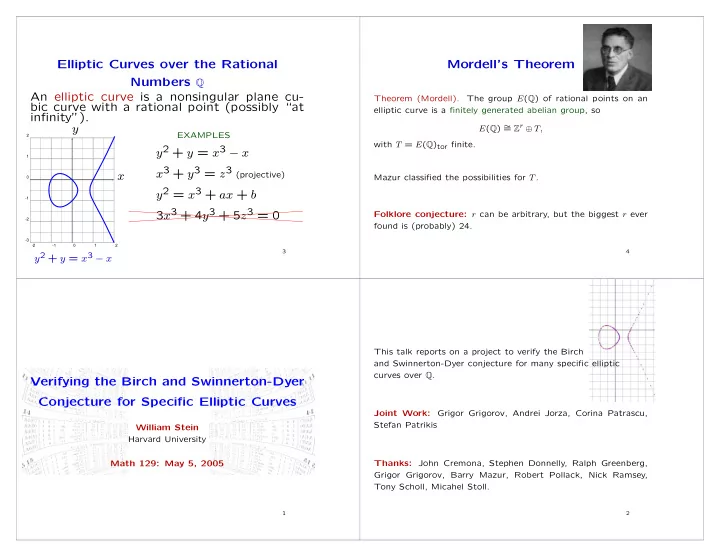
Elliptic Curves over the Rational Numbers Q An elliptic curve is a nonsingular plane cu- bic curve with a rational point (possibly “at infinity”).

• 2
• 1

1 2

• 3
• 2
• 1

1 2

x y

y2 + y = x3 − x

EXAMPLES

y2 + y = x3 − x x3 + y3 = z3 (projective) y2 = x3 + ax + b 3x3 + 4y3 + 5z3 = 0

3

Mordell’s Theorem

Theorem (Mordell). The group E(Q) of rational points on an elliptic curve is a finitely generated abelian group, so E(Q) ∼ = Zr ⊕ T, with T = E(Q)tor finite. Mazur classified the possibilities for T. Folklore conjecture: r can be arbitrary, but the biggest r ever found is (probably) 24.

4

Conjectures Proliferated

“The subject of this lecture is rather a special one. I want to de- scribe some computations undertaken by myself and Swinnerton- Dyer on EDSAC, by which we have calculated the zeta-functions

• f certain elliptic curves. As a result of these computations we

have found an analogue for an elliptic curve of the Tamagawa number of an algebraic group; and conjectures have proliferated. [...] though the associated theory is both abstract and techni- cally complicated, the objects about which I intend to talk are usually simply defined and often machine computable; experi- mentally we have detected certain relations between different invariants, but we have been unable to approach proofs of these relations, which must lie very deep.” – Birch 1965

5

The L-Function

Theorem (Wiles et al., Hecke) The following function extends to a holomorphic function on the whole complex plane:

L(E, s) =

• p∤∆

  

1 1 − ap · p−s + p · p−2s

  ·

• p|N

Lp(E, s)

Here ap = p + 1 − #E(Fp) for all p ∤ ∆, where ∆ is divisible by the primes of bad reduction for E. We do not include the factors Lp(E, s) at bad primes here.

6

Real Graph of the L-Series of y2 + y = x3 − x

7

Graph of L-Series of y2 + y = x3 − x

• ✁
• ✂

• ✄ ✝

• ✄ ✝

• ✄ ✝

• ✄ ✝

8

The Birch and Swinnerton-Dyer Conjecture

Conjecture: Let E be any elliptic curve over Q. The order of vanishing of L(E, s) as s = 1 equals the rank of E(Q).

9

The Kolyvagin and Gross-Zagier Theorems

Theorem: If the ordering of vanishing ords=1 L(E, s) is ≤ 1, then the conjecture is true for E.

10

What about Taylor series of L(E, s) around s = 1?

11

Taylor Series

For y2 + y = x3 − x, the Taylor series about 1 is

L(E, s) = 0 + (s − 1)0.3059997 . . . +(s − 1)20.18636 . . . + · · ·

In general, it’s L(E, s) = c0 + c1s + c2s2 + · · · . Big Mystery: Do these Taylor coefficients cn have any deep arith- metic meaning?

12

BSD Formula Conjecture

Let r = ords=1 L(E, s). Then Birch and Swinnerton-Dyer made a famous guess for the first nonzero coefficient cr:

cr = ΩE · RegE ·

• p|N tp

#E(Q)2

tor

· #X(E)

• #E(Q)tor – torsion order
• tp – Tamagawa numbers
• ΩE – real volume
• E(R) ωE
• RegE – regulator of E
• X(E) = Ker(H1(Q, E) →

v H1(Qv, E))

– Shafarevich-Tate group

13

What about cr+1, cr+2, etc? I think nobody has even a wild and crazy guess for an interpretation of these.

They are probably not “periods” like cr is, so perhaps should not have any nice interpretation...

14

Motivating Problem 1

Motivating Problem 1. For specific curves, compute every quantity appearing in the BSD formula conjecture in practice. NOTE: This is not meant as a theoretical problem about computability, though by compute we mean “compute with proof.”

15

Status

• 1. When ran = ords=1 L(E, s) ≤ 3, then we can compute ran.

Open Problem: Show that ran ≥ 4 for some elliptic curve.

• 2. “Relatively easy” to compute #E(Q)tor, cp, ΩE.
• 3. Computing RegE essentially same as computing E(Q); inter-

esting and sometimes very difficult.

• 4. Computing #X(E) is currently very very difficult.

Theorem (Kolyvagin): ran ≤ 1 = ⇒ X(E) is finite (with bounds) Open Problem: Prove that X(E) is finite for some E with ran ≥ 2.

16

Victor Kolyvagin

Kolyvagin’s work on Euler systems is crucial to our project.

17

Motivating Problem 2: Cremona’s Book

Motivating Problem 2. Prove BSD for every elliptic curve

• ver Q of conductor at most 1000, i.e., in Cremona’s book.
• 1. By Tate’s isogeny invariance of BSD, it suffices to prove BSD

for each optimal elliptic curve of conductor N ≤ 1000.

• 2. Rank part of the conjecture has been verified by Cremona

for all curves with N ≤ 40000.

• 3. All of the quantities in the conjecture, except for #X(E/Q),

have been computed by Cremona for conductor ≤ 40000.

• 4. Cremona (Ch. 4, pg. 106): We have 2 ∤ #X(E) for all
• ptimal curves with conductor ≤ 1000 except 571A, 960D,

and 960N. So we can mostly ignore 2 henceforth.

18

John Cremona

John Cremona’s software and book are crucial to our project.

19

The Four Nontrivial X’s

Conclusion: In light of Cremona’s book and the above results, the problem is to show that X(E) is trivial for all but the fol- lowing four optimal elliptic curves with conductor at most 1000: Curve a-invariants X(E)? 571A [0,-1,1,-929,-105954] 4 681B [1,1,0,-1154,-15345] 9 960D [0,-1,0,-900,-10098] 4 960N [0,1,0,-20,-42] 4 We first deal with these four.

20

Divisor of Order:

• 1. Using a 2-descent we see that 4 | #X(E) for 571A, 960D,

960N.

• 2. For E = 681B: Using visibility (or a 3-descent) we see that

9 | #X(E).

21

Multiple of Order:

• 1. For E = 681B, the mod 3 representation is surjective, and

3 || [E(K) : yK] for K = Q(√−8), so Kolyvagin’s theorem implies that #X(E) = 9, as required.

• 2. Kolyvagin’s theorem and computation

= ⇒ #X(E) = 4? for 571A, 960D, 960N.

• 3. Using MAGMA’s FourDescent command, we compute Sel(4)(E/Q)

for 571A, 960D, 960N and deduce that #X(E) = 4. (Note: MAGMA Documentation currently misleading.)

22

The Eighteen Optimal Curves of Rank > 1

There are 18 curves with conductor ≤ 1000 and rank > 1 (all have rank 2): 389A, 433A, 446D, 563A, 571B, 643A, 655A, 664A, 681C, 707A, 709A, 718B, 794A, 817A, 916C, 944E, 997B, 997C For these E nobody currently knows how to show that X(E) is finite, let alone trivial. (But mention, e.g., p-adic L-functions.) Motivating Problem 3: Prove the BSD Conjecture for all el- liptic curve over Q of conductor at most 1000 and rank ≤ 1.

23

SECRET MOTIVATION: Our actual motivation is to unify and extend results about BSD and algorithms for elliptic curves. Also, the computations give rise to many surprising and inter- esting examples.

Our Goal

• There are 2463 optimal curves of conductor at most 1000.
• Of these, 18 have rank 2, which leaves 2445 curves.
• Of these, 2441 are conjectured to have trivial X.

Thus our goal is to prove that #X(E) = 1 for these 2441 elliptic curves.

24

Our Strategy

• 1. [Find an Algorithm] Based on deep work of Kolyvagin,

Kato, et al. Input: An elliptic curve over Q with ran ≤ 1. Output: B ≥ 1 such that if p ∤ B, then p ∤ #X(E).

• 2. [Compute] Run the algorithm on our 2441 curves.
• 3. [Reducible] If E[p] is reducible say nothing.

25

Kolyvagin Bound on #X(E)

INPUT: An elliptic curve E over Q with ran ≤ 1. OUTPUT: Odd B ≥ 1 such that if p ∤ 2B, then p ∤ #X(E/Q).

• 1. [Choose K] Choose a quadratic imaginary field K = Q(

√ D) with certain properties, such that E/K has analytic rank 1. Assume Q(E[p]) has degree # GL2(Fp).

• 2. [Compute Mordell-Weil]

(a) If r = 0, compute generator z for ED(Q) mod torsion. (b) If r = 1, compute generator z for E(Q) mod torsion.

26

• 3. [Index of Heegner point] Compute the “Heegner point”

yK ∈ E(K) associated to K. This is a point that comes from the “modularity” map X0(N) → E.

• 4. [Finished] Output B = I·A, where A is the product of primes

such that Q(E[p]) has degree less than # GL2(Fp). Theorem (Kolyvagin): p ∤ 2B = ⇒ p ∤ #X(E/Q).