How to estimate the GW-signal emitted by an evolv- ing system: THE - PDF document

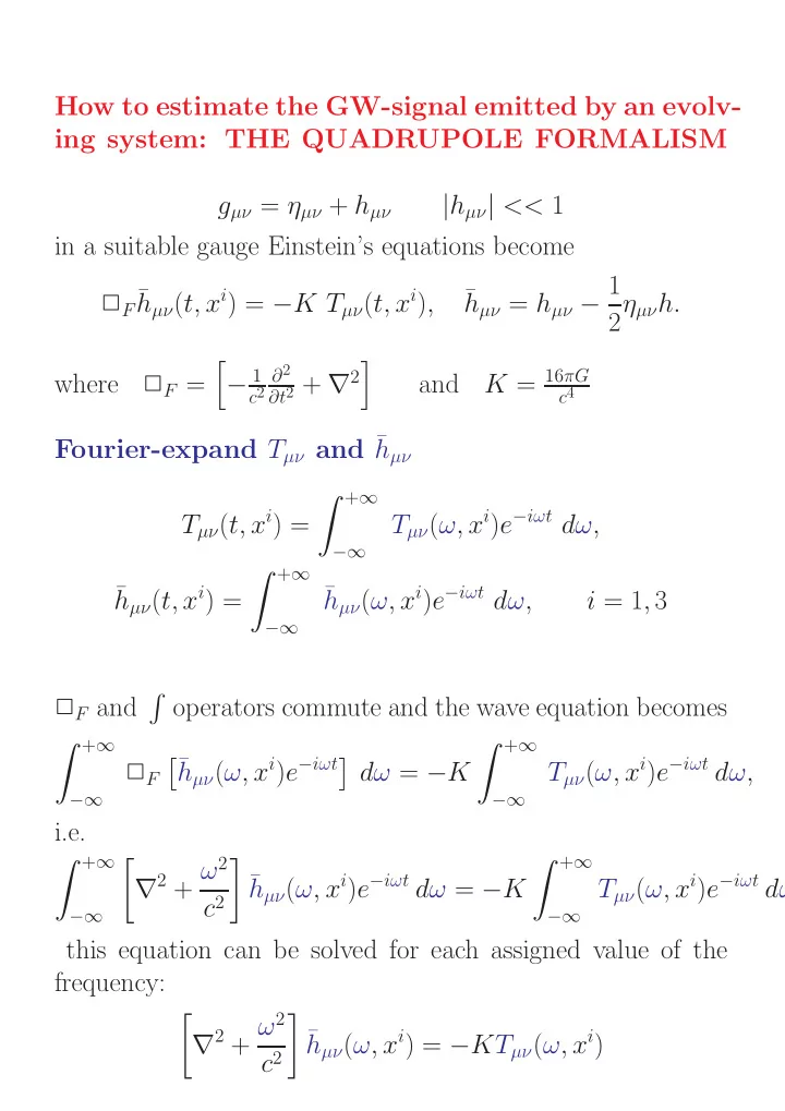
How to estimate the GW-signal emitted by an evolv- ing system: THE QUADRUPOLE FORMALISM g µν = η µν + h µν | h µν | << 1 in a suitable gauge Einstein’s equations become h µν = h µν − 1 ✷ F ¯ ¯ h µν ( t, x i ) = − K T µν ( t, x i ) , 2 η µν h. � ∂t 2 + ∇ 2 � ∂ 2 K = 16 πG − 1 where ✷ F = and c 2 c 4 Fourier-expand T µν and ¯ h µν � + ∞ T µν ( ω, x i ) e − iωt dω, T µν ( t, x i ) = −∞ � + ∞ h µν ( ω, x i ) e − iωt dω, ¯ ¯ h µν ( t, x i ) = i = 1 , 3 −∞ � ✷ F and operators commute and the wave equation becomes � + ∞ � + ∞ T µν ( ω, x i ) e − iωt dω, � ¯ h µν ( ω, x i ) e − iωt � dω = − K ✷ F −∞ −∞ i.e. � + ∞ � + ∞ ∇ 2 + ω 2 � � h µν ( ω, x i ) e − iωt dω = − K T µν ( ω, x i ) e − iωt dω ¯ c 2 −∞ −∞ this equation can be solved for each assigned value of the frequency: ∇ 2 + ω 2 � � ¯ h µν ( ω, x i ) = − KT µν ( ω, x i ) c 2

SLOW-MOTION APPROXIMATION We shall solve the wave equation ∇ 2 + ω 2 � � ¯ h µν ( ω, x i ) = − KT µν ( ω, x i ) c 2 assuming that the region where the source is confined | x i | ≤ ǫ ǫ ǫ, T µν � = 0 , is much smaller than the wavelenght of the emitted radiation λ GW = 2 πc ω 2 πc ω >> ǫ ǫ ǫ → ǫ ǫ ǫ ω << c → v << c The wave equation will be solved inside and outside the source, and the two solutions will be matched on the source boundary

Let us first integrate the equations OUTSIDE the source ∇ 2 + ω 2 � � ¯ h µν ( ω, x i ) = 0 c 2 In polar coordinates, the Laplacian operator is ∂ 2 � � � � ∇ 2 = 1 ∂ r 2 ∂ 1 ∂ sen θ ∂ 1 + + r 2 sen θ r 2 sen 2 θ r 2 ∂r ∂r ∂θ ∂θ ∂φ 2 The simplest solution does not depend on φ and θ h µν ( ω, r ) = A µν ( ω ) c r + Z µν ( ω ) e i ω e − i ω ¯ c r , r r This solution represents a spherical wave, with an ingoing part ( ∼ e − i ω c r ), and an outgoing ( ∼ e i ω c r ) part. Since we are interested only in the wave emitted from the source, we set Z µν = 0 , and the solution becomes h µν ( ω, r ) = A µν ( ω ) e i ω ¯ c r r This is the solution outside the source, and on its boundary x = ǫ How do we find A µν ( ω )? To answer this question we need to integrate the equations inside the source

INSIDE THE SOURCE ∇ 2 + ω 2 � � ¯ h µν ( ω, x i ) = − KT µν ( ω, x i ) c 2 This equation can be solved for each assigned value of the in- dices µ, ν. Let us integrate each term over the source volume ∇ 2 + ω 2 � � � � ¯ h µν ( ω, x i ) d 3 x = − K T µν ( ω, x i ) d 3 x A ) c 2 V V � � ∇ 2 ¯ div [ � ∇ ¯ h µν d 3 x = h µν ] d 3 x 1) V V � d � � � k � ∇ ¯ � ¯ ǫ 2 = h µν dS k ≃ 4 π ǫ ǫ h µν dr r = ǫ ǫ ǫ S � d � A µν ( ω ) e i ω c r ǫ 2 = 4 π ǫ ǫ dr r ǫ r = ǫ ǫ � � iω � � − A µν c r + A µν r 2 e i ω e i ω c r ǫ 2 = 4 π ǫ ǫ ∼ − 4 π A µν ( ω ) r c ǫ r = ǫ ǫ ǫ neglecting all terms of order ≥ ǫ ǫ � ∇ 2 ¯ h µν ( ω, x i ) d 3 x ≃ − 4 π A µν ( ω ) V Eq. A ) now becomes ω 2 � � c 2 ¯ h µν ( ω, x i ) d 3 x = − K T µν ( ω, x i ) d 3 x − 4 π A µν ( ω )+ V V

ω 2 h µν ( ω, x i ) d 3 x � ω 2 � 4 c 2 ¯ c 2 | ¯ ǫ 3 h µν | max 3 πǫ ǫ negligible V The final solution inside the source gives � K = 16 πG T µν ( ω, x i ) d 3 x − 4 πA µν ( ω ) = − K c 4 V A µν ( ω ) = K � T µν ( ω, x i ) d 3 x = 4 G � T µν ( ω, x i ) d 3 x 4 π c 4 V V SUMMARIZING: By integrating the wave equation outside the source we find h µν ( ω, r ) = A µν ( ω ) e i ω ¯ c r r by integrating over the source volume we find A µν ( ω ) = 4 G � T µν ( ω, x i ) d 3 x, c 4 V therefore c 4 · e iω r h µν ( ω, r ) = 4 G � c ¯ T µν ( ω, x i ) d 3 x, r V or, in terms of the outgoing coordinate ( t − r c , x i ) h µν ( t, r ) = 4 G � T µν ( t − r ¯ c, x i ) d 3 x . c 4 r · V

h µν ( t, r ) = 4 G � T µν ( t − r ¯ c, x i ) d 3 x, c 4 r V We shall now simplify the integral over T µν . We are in flat spacetime, therefore ∂ 1 ∂tT µ 0 = − ∂ ∂ ∂x ν T µν = 0 , ∂x k T µk , → k = 1 , 3 c Integrate over the source volume: � 1 ∂ � ∂ ∂tT µ 0 d 3 x = − ∂x k T µk d 3 x ; c V V Apply Gauss’s theorem to the R.H.S. � ∂ � ∂x k T µk d 3 x = T µk dS k V S where S is the surface which encloses V . � T µk dS k = 0 , and On S , T µν = 0 , therefore S 1 ∂ � T µ 0 d 3 x = 0 , c ∂t V i.e. � T µ 0 d 3 x = const, h µ 0 = const. ¯ → V Since we are interested in the time-dependent part of the field, we put ¯ h µ 0 ( t , r ) = ¯ h µ 0 ( t , r ) = 0 ; (this condition is automatically satisfied when transforming to the TT-gauge)

To simplify the space components of ¯ h µν : h ik ( t, r ) = 4 G � T ik ( t − r ¯ c, x i ) d 3 x, i, k = 1 , 3 c 4 r V we shall use the Tensor-Virial Theorem Let us consider the space components of the conservation low ∂T µν ∂T n 0 + ∂T ni 1 ) 1 ∂x ν = 0 → ∂x i = 0 , n, i = 1 , 3 c ∂t multiply 1) by x k and integrate over the volume ∂T ni 1 ∂ � � T n 0 x k dx 3 = − ∂x i x k dx 3 c ∂t V V T ni x k � �� � � T ni ∂x k � ∂x k ∂ � � dx 3 − ∂x i = δ k ∂x i dx 3 = − i ∂x i V V � � T ni x k � T nk dx 3 � = − dS i + S V � T ni x k � � as before, dS i = 0 , therefore S 1 ∂ � � T n 0 x k dx 3 = T nk dx 3 c ∂t V V Since T nk is symmetric in n and k , 1 ∂ � � T k 0 x n dx 3 = T kn dx 3 c ∂t V V and adding the two we get

1 ∂ � � T n 0 x k + T k 0 x n � dx 3 = T nk dx 3 . � 2 c ∂t V V

We shall now use the 0- component of the conservation low: ∂T 0 ν + ∂T 0 i ∂T 00 2 ) 1 ∂x ν = 0 → ∂x i = 0 c ∂t multiply 2) by x k x n and integrate ∂T 0 i 1 ∂ � � T 00 x k x n dx 3 = − ∂x i x k x n dx 3 c ∂t V V T 0 i x k x n � �� � T 0 i ∂x k ∂x i x n + T 0 i x k ∂x n ∂ � � � dx 3 − = − ∂x i ∂x i V V � � T 0 i x k x n � T 0 k x n + T 0 n x k � dx 3 � � = − dS i + S V as before, the first integral vanishes, and 1 ∂ � � T 00 x k x n dx 3 = T 0 k x n + T 0 n x k � dx 3 . � c ∂t V V Let us differenciate with respect to x 0 = ct : ∂ 2 1 � T 00 x k x n dx 3 = 1 ∂ � T 0 k x n + T 0 n x k � dx 3 � c 2 ∂t 2 c ∂t V V and since we just found 1 ∂ � � T n 0 x k + T k 0 x n � dx 3 = T nk dx 3 , � 2 c ∂t V V finally ********************************************** ∂ 2 V T kn dx 3 = 1 � T 00 x k x n dx 3 . � 2 c 2 ∂t 2 V

∂ 2 V T kn dx 3 = 1 � T 00 x k x n dx 3 . � 2 c 2 ∂t 2 V The quantity 1 � T 00 x k x n dx 3 is the Quadrupole Mo- c 2 V ment Tensor of the system q kn ( t ) = 1 � T 00 ( t, x i ) x k x n dx 3 , (1) c 2 V and it is a function of time only. In conclusion d 2 � T kn ( t, x i ) dx 3 = 1 dt 2 q kn ( t ) 2 V and since h kn ( t, r ) = 4 G � T kn ( t − r ¯ c, x i ) d 3 x, c 4 r · V we finally find h µ 0 = 0 ,  ¯ µ = 0 , 3     (2) � d 2 h kn ( t, r ) = 2 G dt 2 q kn ( t − r � ¯  c 4 r · c ) , k, n = 1 , 3    This is the gravitational wave emitted by a mass- energy system evolving in time

h µ 0 = 0 ,  ¯ µ = 0 , 3     (3) � d 2 � h kn ( t, r ) = 2 G dt 2 q kn ( t − r ¯  c 4 r · c ) , k, n = 1 , 3    NOTE THAT G c 4 ∼ 8 · 10 − 50 s/g cm 1) GW are extremely weak! 2) We are not yet in the TT-gauge 3) these equations are derived on very strong assumptions: one is that T µν,ν = 0 , i.e. the motion of the bodies is dominated by non-gravitational forces. However , and remarkably, the result depends only on the sources motion and not on the forces acting on them.

Gravitational radiation has a quadrupolar nature. A system of accelerated charged particles has a time-varying dipole moment � � d EM = q i � r i i and it will emit dipole radiation, the flux of which depends on the second time derivative of � d EM . For an isolated system of masses we can define a gravitational dipole moment � � d G = m i � r i , i which satisfies the conservation law of the total momentum of an isolated system d � d G = 0 . dt For this reason, gravitational waves do not have a dipole contribution. It should be stressed that for a spherical or axisymmetric dis- tribution of matter (or energy) the quadrupole moment is a constant , even if the body is rotating: thus, a spherical or axisymmetric star does not emit gravitational waves; similarly, a star which collapses in a perfectly spherically sym- metric way has a vanishing q ik and does not emit gravitational waves.

To produce waves we need a certain degree of asym- metry, as it occurs for instance in the non-radial pulsations of stars, in a non spherical gravitational collapse, in the coalescence of massive bodies etc.